How to compute the symbol error rate rate of an m-FSK modulation is something that comes up in a variety of situations, since the math is the same in any setting in which the symbols are orthogonal (so it also applies to some spread spectrum modulations). I guess this must appear somewhere in the literature, but I can never find this result when I need it, so I have decided to write this post explaining the math.
Here I show an approach that I first learned from Wei Mingchuan BG2BHC two years ago during the Longjiang-2 lunar orbiter mission. While writing our paper about the mission, we wanted to compute a closed expression for the BER of the LRTC modulation used in the uplink (which is related to \(m\)-FSK). Using a clever idea, Wei was able to find a formula that involved an integral of CDFs and PDFs of chi-squared distributions. Even though this wasn’t really a closed formula, evaluating the integral numerically was much faster than doing simulations, specially for high \(E_b/N_0\).
Recently, I came again to the same idea independently. I was trying to compute the symbol error rate of \(m\)-FSK and even though I remembered that the problem about LRTC was related, I had forgotten about Wei’s formula and the trick used to obtain it. So I thought of something on my own. Later, digging through my emails I found the messages Wei and I exchanged about this and saw that he had arrived to the same idea and formula. Maybe the trick was in the back of my mind all the time.
Due to space constraints, the BER formula for LRTC and its mathematical derivation didn’t make it into the Longjiang-2 paper. Therefore, I include a small section below with the details.
Setting
We will assume that the symbols sent by the transmitter are a set of orthonormal vectors \(\{v_1,\ldots,v_m\}\) in a space which is either \(\mathbb{C}^N\) in the discrete time case, or \(\mathbb{C}^{[0,T]}\), the set of functions from the interval \([0,T]\) to \(\mathbb{C}\), in the continuous time case (though the space where these vectors live is not so important, as long as one is able to define white Gaussian noise on it, in the precise sense given below).
Note that this is the case in \(m\)-FSK whenever the tones are orthogonal, meaning that the frequency spacing between each pair of tones is an integer multiple of the symbol rate, and there is no pulse shape filtering. In particular this setting does not cover GFSK.
The transmitter sends a vector \(v_k\) with \(1 \leq k \leq m\) and the receiver receives that vector plus noise, which we denote by \(w = v_k + n\). Without loss of generality, we will assume below that \(k = 1\).
The noise \(n\) will be assumed to be Gaussian and white, so that in particular, the scalar products \(\langle n, v_1\rangle\), …, \(\langle n, v_m\rangle\) are independent complex normal random variables with mean zero and variance \(\sigma^2 = (E_s/N_0)^{-1}\).
Coherent detection
In the case of coherent detection, the receiver performs the maximum-likelihood detection of the symbols. It computes \(\text{Re} \langle w, v_j\rangle\) for \(j = 1,…,m\), and chooses as output the symbol \(v_j\) that maximizes this expression. Since \(w = v_1 + n\), we have\[\text{Re} \langle w, v_1\rangle = 1 + \text{Re}\langle n, v_1\rangle.\]For \(j \geq 2\) we have\[\text{Re}\langle w, v_j\rangle = \text{Re}\langle n, v_j\rangle.\]The real parts of the scalar products involving the noise are distributed as independent real normal variables with mean zero and variance \(\sigma^2/2\). Dividing by \(\sigma/\sqrt{2}\) and putting \(\alpha = \sqrt{2E_s/N_0}\), we see that the probability of correct detection (which is \(1-\mathrm{SER}\), where \(\mathrm{SER}\) denotes the symbol error rate) is equal to the probability that \(\alpha + N_1\) is greater than the maximum of \(N_2, \ldots, N_m\), where \(N_1,\ldots, N_m\) are independent real normal variables with zero mean and variance one. This can be computed using conditional expectation as we indicate now.
By conditioning to the fact that \(N_1 = t – \alpha\), we have to compute\[\begin{split}1-\mathrm{SER} &= E[\mathbb{P}(N_2 \leq t, \ldots, N_m \leq t\, |\, N_1 = t – \alpha)] \\ &= E[\mathbb{P}(N_2 \leq t\, |\, N_1 = t-\alpha)^{m-1}] \\ &= \int_{-\infty}^{+\infty} F(t)^{m-1} f(t-\alpha)\, dt,\end{split}\]where \(F\) denotes the cumulative distribution function of the normal distribution and \(f(t) = e^{-t^2/2}/\sqrt{2\pi}\) denotes the probability density function of the normal distribution. The second equality above is due to the fact that \(N_2,\ldots,N_m\) are independent and equidistributed.
The integral above cannot be evaluated in closed form, so we can write the symbol error probability for the coherent detection case as\[\mathrm{SER} = 1 – \int_{-\infty}^{+\infty} F(t)^{m-1} f\left(t-\sqrt{2E_s/N_0}\right)\, dt.\]
Non-coherent detection
In the non-coherent detection case, the receiver computes the powers \(|\langle w, v_j\rangle|^2\) for \(j = 1,…,m\) and chooses as output the vector \(v_j\) that maximizes this expression. The calculations for this case are similar to those for the coherent detection, but now we have chi-squared variables instead of normals.
Indeed, the power\[|\langle w, v_1\rangle|^2 = |1 + \langle n, v_1\rangle|^2\]equals \(\sigma^2 X_1\), where \(X_1\) is a non-central chi-squared variable with two degrees of freedom and non-centrality parameter \(\lambda = 2E_s/N_0\). The remaining powers\[|\langle w, v_j\rangle|^2 = |\langle n, v_j\rangle |^2\]are equal to \(\sigma^2 X_j\), where \(X_j\) are central chi-squared variables with two degrees of freedom. Moreover, the variables \(X_1, X_2,\ldots, X_m\) are independent.
By conditioning to \(X_1 = t\), we have that the probability of correct detection equals\[\begin{split}1-\mathrm{SER}&= E[\mathbb{P}(X_2 \leq t, \ldots, X_m \leq t\, |\, X_1 = t)] \\ &= E[\mathbb{P}(X_2 \leq t\, |\, X_1 = t)^{m-1}] \\ &= \int_{-\infty}^{+\infty} G(t)^{m-1} g_\lambda(t)\, dt.\end{split}\]Here \(G(t)\) denotes the cumulative distribution function of a central chi-squared variable with two degrees of freedom and \(g_\lambda(t)\) denotes the probability density function of a non-central chi-squared variable with two degrees of freedom and non-centrality parameter \(\lambda = 2E_s/N_0\).
Thus, the symbol error probability can be computed as\[\mathrm{SER}=1 – \int_{-\infty}^{+\infty} G(t)^{m-1} g_{2E_s/N_0}(t)\, dt.\]
LRTC
The LRTC (low-rate telecommand) modulation used in the Longjiang-1/2 mission could be described as a 2-FSK modulation where the tones are spread with a GMSK PN code. Alternatively, it can be described as transmitting a GMSK PN code either on one of two frequencies, with the symbol encoded by the choice of frequency. After de-spreading the GMSK PN code, what remains is a 2-FSK modulation. The tone separation is much larger than the symbol rate. In order to handle frequency offsets due to Doppler, an FFT whose bin width equals the symbol rate is done, and the symbol is decided according to which FFT bin has maximum power. Half of the FFT bins (the ones corresponding to negative frequencies) correspond to symbol 0, while the remaining half correspond to symbol 1.
Here the vectors \(v_j\) are the complex exponentials corresponding to the tones used by the FFT,\[v_j[l] = e^{2\pi i l/m},\quad l=1,…,m.\]We assume that the received tone lies exactly in one FFT bin, so the transmitted vector is one of these tones, and we can assume again that the transmitted vector is \(v_1\) without loss of generality.
The statistics are exactly as in the \(m\)-FSK non-coherent detection case, but now we consider that a bit error happens whenever the \(v_j\) that maximizes \(|\langle w, v_j\rangle|^2\) has \(j > m/2\) (whereas in the \(m\)-FSK non-coherent detection case we had \(j \geq 2\)).
The probability that there is no bit error can be computed in the following way. We denote by \(Z\) the event corresponding to \(X_1 \geq X_2\), \(X_1 \geq X_3\), …, \(X_1 \geq X_m\). There are two possible ways in which we can decode successfully. Either \(Z\) happens, in which case we will choose the correct bin that corresponds to the transmitted tone, and hence obtain the correct bit, or either \(Z\) does not happen, but among the variables \(X_2,\ldots,X_m\) the variable \(X_j\) with maximum value has \(j \leq m/2\). In this latter case we do not choose the correct bin but still choose a bin that decodes to the correct bit.
The probability that \(Z\) happens is just what we have computed in the non-coherent detection case, so\[\mathbb{P}(Z) = \int_{-\infty}^{+\infty} G(t)^{m-1} g_{2E_s/N_0}(t).\] If we condition to \(\neg Z\), the probability that among \(X_2,\ldots,X_m\) the variable with maximum value has \(j \leq m/2\) is just \((m/2-1)/(m-1)\), since we have \(m-1\) independent and identically distributed variables which are also independent of \(\neg Z\), so the probability that the maximum of them is one of the first \(m/2-1\) is simply \((m/2-1)/(m-1)\).
Therefore, the probability of decoding correctly is\[\begin{split}1-\mathrm{BER}&=\mathbb{P}(Z) + \frac{m/2-1}{m-1}\mathbb{P}(\neg Z) = \mathbb{P}(Z) + \frac{m/2-1}{m-1}(1-\mathbb{P}(Z))\\ &= \frac{m/2-1}{m-1} + \frac{m}{2m-2}\mathbb{P}(Z).\end{split}\]Hence, the bit error rate is\[\begin{split}\mathrm{BER} &= 1-\frac{m/2-1}{m-1} – \frac{m}{2m-2}\mathbb{P}(Z) = \frac{m}{2m-2}[1 – \mathbb{P}(Z)] \\ &= \frac{m}{2m-2}\left[1 – \int_{-\infty}^{+\infty} G(t)^{m-1} g_{2E_s/N_0}(t)\, dt\right].\end{split}\]
A word on bit error rate
In the above we have concerned ourselves with the symbol error rate. When \(m = 2^b\), so that \(b\) bits are encoded in each symbol, we can easily calculate the bit error rate from the knowledge of the symbol error rate. In fact, if we denote by \(B\) the number of bit errors that occur in a symbol (so that \(B\) is a random variable), we have\[BER = \frac{1}{b}E[B].\]Now, conditioned to the fact that \(B \geq 1\), i.e., that there is a symbol error, we see that all the wrong symbols are equiprobable. Since for \(l=1,\ldots,b\) there are \({b \choose l}\) symbols with exactly \(l\) bit errors, we have,\[\begin{split}E[B] &= \mathbb{P}(B \geq 1)E[B | B\geq 1] = \mathrm{SER}\frac{1}{2^b -1}\sum_{l=1}^b l {b \choose l} \\ &= \mathrm{SER}\frac{1}{2^b-1}\frac{b}{2}2^b = \mathrm{SER}\frac{b 2^{b-1}}{2^b-1}.\end{split}\]Here we have used\[\sum_{l=0}^b l {b \choose l} = \frac{b}{2}2^b,\]which is a well-known identity related to the expectation of a binomial distribution.
We conclude that\[\mathrm{BER} = \frac{2^{b-1}}{2^b-1}\mathrm{SER} = \frac{m}{2m-2}\mathrm{SER}.\]
We see that we have arrived to the same expression as for the BER of LRTC, which equals the SER of non-coherent detection of \(m\)-FSK multiplied by the factor \(\frac{m}{2m-2}\). In fact, there is a nice relation between the BER of \(m\)-FSK and the BER of LRTC. If we encode the words of \(b\) bits onto the set of symbols in such a way that the symbols \(j=1,\ldots,m/2\) have 0 as their MSB and the symbols \(j=m/2+1,\ldots,m\) have 1 as their MSB, we see that LRTC is equivalent to \(m\)-FSK but only using the MSB of each symbol. Thus, the BER of LRTC is equal to the BER of the MSB of \(m\)-FSK. But the BER of the MSB is equal to the overall BER of \(m\)-FSK, since as remarked above, when there is a symbol error, all the wrong symbols are equiprobable.
Simulations
It is worth to do some simulations to verify that the formulas given above are correct. These are done in this Jupyter notebook. The resulting plot is shown here. It compares the curves obtained by evaluating the formulas with simulations done in steps of 0.5 dB of \(E_s/N_0\). The formulas and simulations agree very well, as expected.
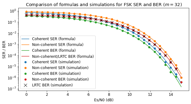
Note that the LRTC BER and the non-coherent \(m\)-FSK BER coincide, as we have explained above.
Hello,
the above relation between BER and SER is not valid for a M-PSK modulation because, in case of a symbols error, it’s more probable to decide for an adjacent symbol?
What is the exact relation in case of M-PSK modulation?
Thanks.
Hi Michele, indeed these results are not applicable to m-PSK.
I think that the symbol error rate of m-PSK can be computed easily in terms of an integral involving the error function (think about the probability that a circularly symmetric complex Gaussian with mean 1 and a given variance falls in the sector given by the complex numbers with arguments between -2π/m and 2π/m).
The bit error rate seems much more tricky. There are at least two possible ways in which one could define the bit error rate, and maybe they give different results:
1. Given a received symbol, pick the most likely constellation symbol, and get the corresponding bit position in the word encoded by this symbol. There is a bit error if the bit in this position does not match the transmitted bit.
2. Given a received symbol, compute its log-likelihood ratio. There is a bit error if the hard-decision on the log-likelihood ratio does not match the transmitted bit.
I’m not even sure if the result of approach 2 depends on the SNR.
Something to keep in mind is that in m-PSK each of the bits tend to have different bit error rates. See for instance Figure 7 in https://ipnpr.jpl.nasa.gov/progress_report/42-184/184D.pdf