Chang’e 5 LOI-2 observed with Allen Telescope Array

If you follow me on Twitter you’ll probably have seem that lately I’m quite busy with the Chang’e 5 mission, doing observations with Allen Telescope Array as part of the GNU Radio activities there and also following what other people such as Scott Tilley VE7TIL, Paul Marsh M0EYT, r00t.cz, Edgar Kaiser DF2MZ, USA Satcom, and even AMSAT-DL at Bochum are doing with their own observations. I have now a considerable backlog of posts to write, recordings to share and data to process. Hopefully I’ll be able to keep a steady stream of information coming out.

In this post I study the observation I did with Allen Telescope Array last Sunday 2019-11-29. During the observation, I was tweeting live the most interesting events. The observation is approximately 3 hours long and contains the LOI-2 (lunar orbit injection) manoeuvre near its end. LOI-2 was a burn that circularized the elliptical lunar orbit into an orbit with a height of approximately 207km over the lunar surface.

The observation was done on the four X-band low data rate telemetry signals: 8463.7 MHz, 8471.2 MHz, 8478.6 MHz, and 8486.2 MHz. The first and third of these frequencies are know to correspond to the lander, while the other two correspond to the orbiter (this only became clear after the two separated after this observation and the lander lowered its orbit).

The telescope was set up in the following manner. Antenna 1h was used with LO d in the RFCB tuned to 8475 MHz and an IF output of 512 MHz. A USRP N321 digitized the IF at 30.72 Msps. The GNU Radio flowgraph record_2x_ce5.grc channelized and decimated to 240 ksps each of the four frequencies, and recorded IQ data for each of the two linear polarizations X and Y. During the observation, the LO was lowered by 30 kHz on two occasions to prevent the signals from drifting out of their channel’s passband due to Doppler drift.

I am still uploading the IQ recordings to Zenodo, but the files are quite large and the telescope’s internet connection is not very fast. So far I have published the first two frequencies, which can be found at… I’ll update this post when I finish uploading the other two frequencies.

Update 2020-12-09: The two remaining files have been now published. The list of all the files is:

• Chang’e 5 RF recording at 8463.7 MHz with Allen Telescope Array during LOI-2
• Chang’e 5 RF recording at 8471.2 MHz with Allen Telescope Array during LOI-2
• Chang’e 5 RF recording at 8478.6 MHz with Allen Telescope Array during LOI-2
• Chang’e 5 RF recording at 8486.2 MHz with Allen Telescope Array during LOI-2

All the four low data rate signals are PCM/PSK/PM with a subcarrier of 65536 Hz. The two lander frequencies use 2048 baud, while the two orbiter frequencies use 4096 baud. The frames are CCSDS concatenated frames carrying AOS frames of 220 bytes, so that the lander s transmits one frame per second in each of its frequencies and the orbiter transmits two frames per second in each frequency, as I described in my previous post.

I have used the ce5_240k_spectrum.grc flowgraph to compute spectra for each of the recordings. These are then loaded and plotted in a Jupyter notebook to produce the image shown below, which overlays all the four signals using different colours so that the Doppler of each signal can be easily compared.

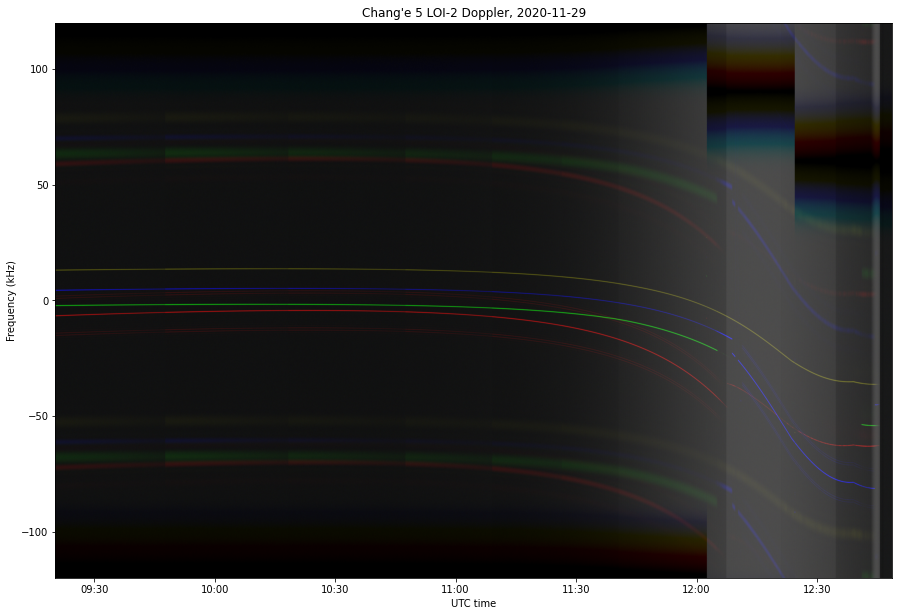
A small vertical offset has been added to each of the signals shown in this plot to prevent them from overlapping. The colours I used are red for 8463.7 MHz, green for 8471.2 MHz, blue for 8478.6 MHz, and yellow for 8486.2 MHz. We can readily see that the data sidebands for the red and blue lander frequencies are thinner than those of the orbiter green and yellow frequencies.

The 30 kHz jumps in the LO have been corrected in this plot, and can be seen because the edges of the passband jump twice near the right hand side of the image. Therefore, any jump seen in the frequency of the signals is due to a ground lock or unlock.

The ground-locked signals can be easily spotted because their Doppler rate is approximately twice as large as that of the other signals and because of two fine carriers at approximately +/- 8 kHz from the main carrier. These carriers come from the uplink signal, as shown in this image of the uplink received via Moonbounce by Paul Marsh. The carriers are actually an idle telecommand signal, which is transmitted constantly, so that when a telecommand frame is transmitted, the spacecraft already is locked to the telecommand subcarrier and data clocks.

This is different to Tianwen-1, for which the telecommand subcarrier is only sent when there is a telecommand frame to be transmitted. Perhaps the reason is that the small round-trip time to Chang’e 5 permits a more real-time way of commanding the spacecraft (for example it is possible to see in the telemetry whether the spacecraft has telecommand lock during a tracking session), while the interaction with Tianwen-1 is necessarily more batch-like.

In this observation, only one of the frequencies is ground-locked at a time, and it’s always either the red or the blue frequency, both of which correspond to the lander. For most of the observation, 8463.7 MHz is the ground-locked frequency. However, shortly after 12:00 UTC the other lander frequency, 8478.6 MHz becomes stronger, most likely due to the changing spacecraft’s attitude, and the ground-locked signal is switched to 8478.6 MHz.

At nearly the same time, the 8471.2 MHz signal, which was strong, becomes heavily attenuated and disappears in the noise, until reappearing shortly after the end of the LOI-2 burn. Probably the attitude required for the retrograde burn placed the antenna for this signal behind the spacecraft’s body.

The LOI-2 burn happened between 12:23 and 12:39 UTC. The beginning of the burn is not easy to see, as it is masked with the large Doppler drift rate. The end of the burn can be easily seen as a kink in the Doppler curve near the end of the observation.

There are more interesting things to see in this plot. During the observation I was hand-tracking by using right ascension and declination coordinates computed from some ephemerides generated by Scott Tilley, and commanding the antenna to change pointing every 10 or 20 minutes (between commands the antenna compensates for the Earth rotation and keeps pointing to the same right ascension and declination). These pointing changes can be seen as changes in the strength of the data sidebands.

As the spacecraft comes closer to the Moon’s disc, the noise floor raises, since the Moon’s thermal noise corresponding to a full Moon enters the dish beam (which has around 0.4 degrees of 3dB beamwidth). At the end of the observation, the Moon goes below the minimum 16.8 degrees that the dish can track and we quickly lose the signal and the Moon noise.

To decode the frames, I’ve taken advantage of the dual polarization recording to improve the SNR. The polarization of each of the signals is elliptical and changes with time, rather than being a fixed circular polarization. Probably this is caused by the antennas being patch-like antennas, which typically are only circularly polarized when seen at a small boresight angle.

Therefore, I have decided to create an “auto-polarization” block that keeps track of the changing polarization, and performs the linear combination of the X and Y polarizations that maximizes the output SNR. This block is still in a prototype stage as an embedded Python block using Numpy for the calculations, but there has been some interest to release this block in a more polished way, since it can be useful for many applications.

The decoder, including the auto-polarization block, is in the ce5_240k.grc GNU Radio flowgraph. The structure of the telemetry decoder is very similar to the Tianwen-1 decoder and the decoders I showed in my “Decoding Interplanetary Spacecraft” workshop at GRCon2020. It uses some blocks from gr-satellites, namely the AGC and the CCSDS deframer blocks. The flowgraph can be seen below. GUI blocks are disabled so that the decoder can run by SSH directly on the GNU Radio server at Allen Telescope Array.

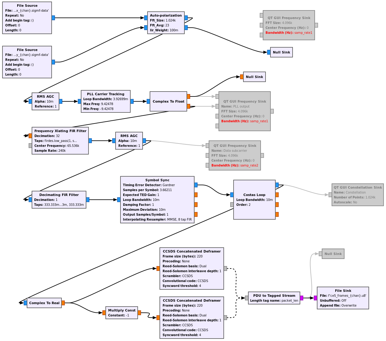
The flowgraph easily accommodates 2048 and 4096 baud by using a decimation of 32 or 16 in the Frequency Xlating FIR Filter, so that everything after this block looks the same regardless of the baudrate.

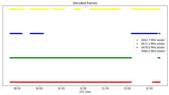
The decoded AOS frames are saved to a file. The files are then loaded and analyzed in this Jupyter notebook. The data files are included with the notebook in the repository. The figure below shows the decoded frames in each signal, using the same colour coding as the waterfall shown above. We see that there are gaps when some of the signals are too weak.

As I already explained in my previous post, the frames are CCSDS AOS frames. The lander frequencies use Spacecraft ID 91, while the orbiter frequencies use Spacecraft ID 108. The two frequencies of each spacecraft transmit exactly the same data simultaneously, so they can be used for diversity reception of the frames. A more interesting exercise would be to try to combine both signals coherently before demodulation, which would give even better results.

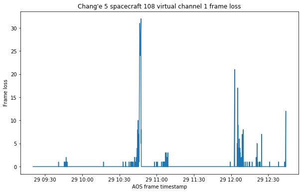
There are two Virtual Channels in use by each of the spacecraft: Virtual Channel 1, which is used to transmit real time telemetry, and Virtual Channel 2, which only sends a few frames sporadically. Since the time intervals where one signal is weak are filled in by the complementary signal (most likely the antennas are placed with this in mind, so that at least one of the two is in a favourable position regardless of the spacecraft’s attitude), we end up losing only a few frames after combining the data from each pair of signals. This is illustrated by the two figures below, which show the number of lost frames versus time.

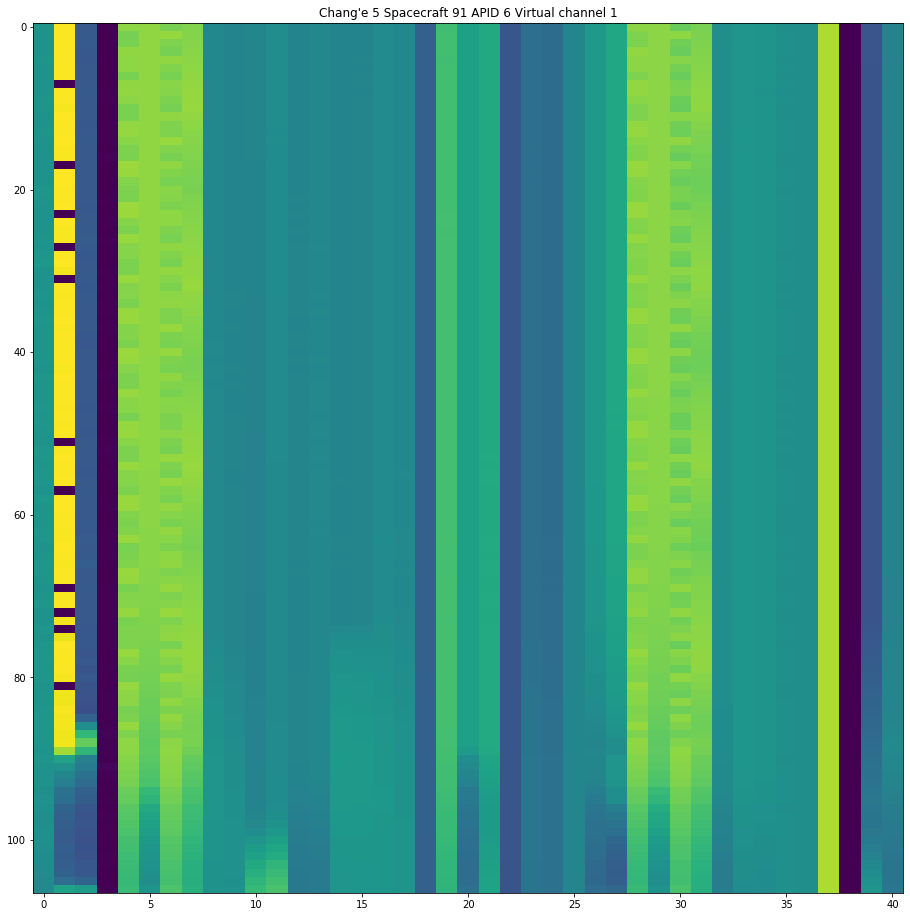
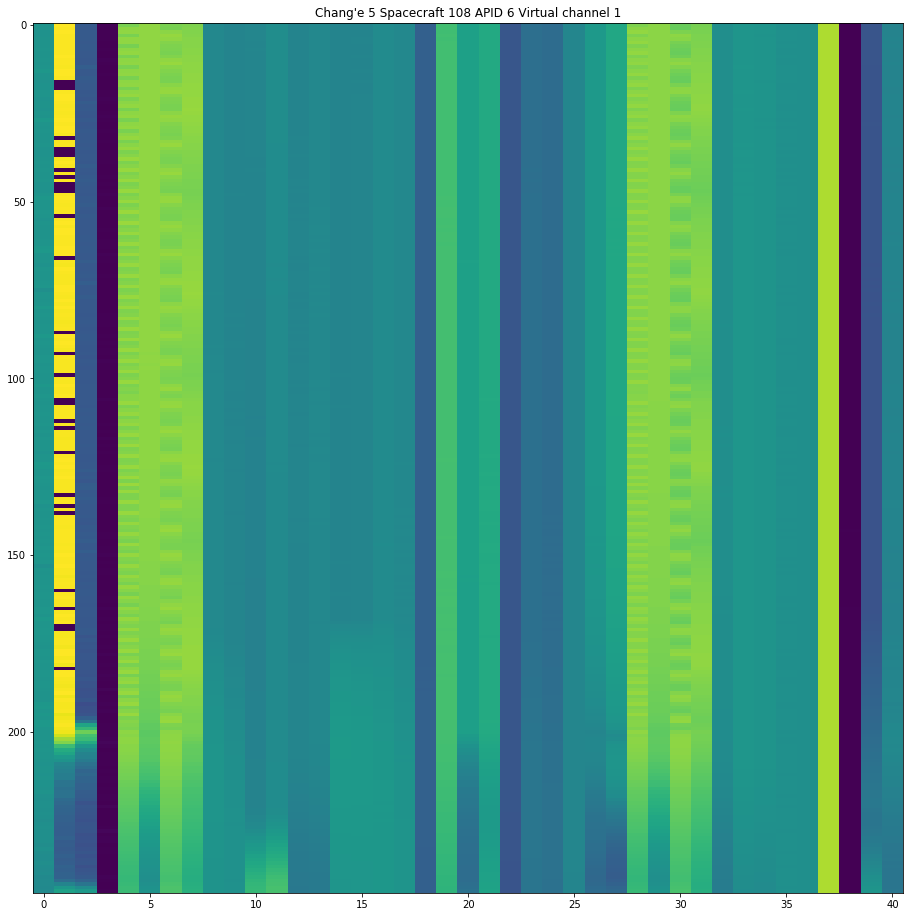
As in the recordings analysed in my previous post, Virtual Channel 1 contains fragmented CCSDS Space Packets using the M_PDU protocol. These Space Packets use a large number of different APIDs. The information sent by Spacecraft 91 and Spacecraft 108 in the Space Packets from Virtual Channel 1 is very similar. The same APIDs are used by both spacecraft, and the structure and contents of each APID is the same, so both spacecraft are sending the same real-time telemetry channels. The only difference is that most of the APIDs in Spacecraft 108 are sampled twice as fast as in Spacecraft 91, since it uses double the baudrate.

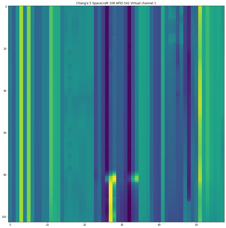
The effects of the LOI-2 burn are clearly visible in many of the APIDs, but still it is not so easy for me to figure out the exact meaning of any of the telemetry channels. The figures below show some of the most interesting APIDs, and compare the data transmitted by each of the spacecrafts.

Some of the channels in APID 542 seem to light up with the LOI-2 burn, and the contents transmitted by both spacecraft seem identical.

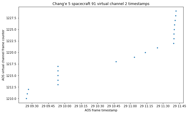
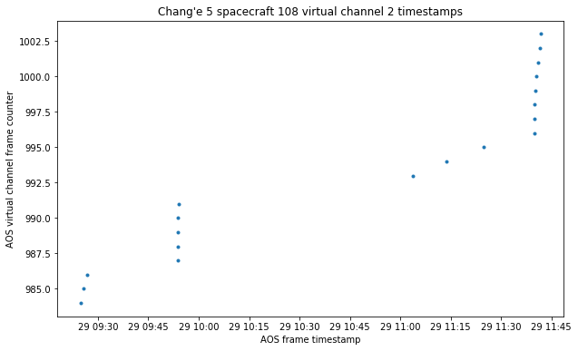
I am not sure what triggers the transmission of these frames. For the first three it might be possible that they are responses to telecommands, since there are telecommands in the telecommand loopback at more or less the same time that these packets are sent. The others do not seem to correspond to telecommands. However, there is a fair amount of telecommands in the loopback, so it is not so easy to try to match things up.

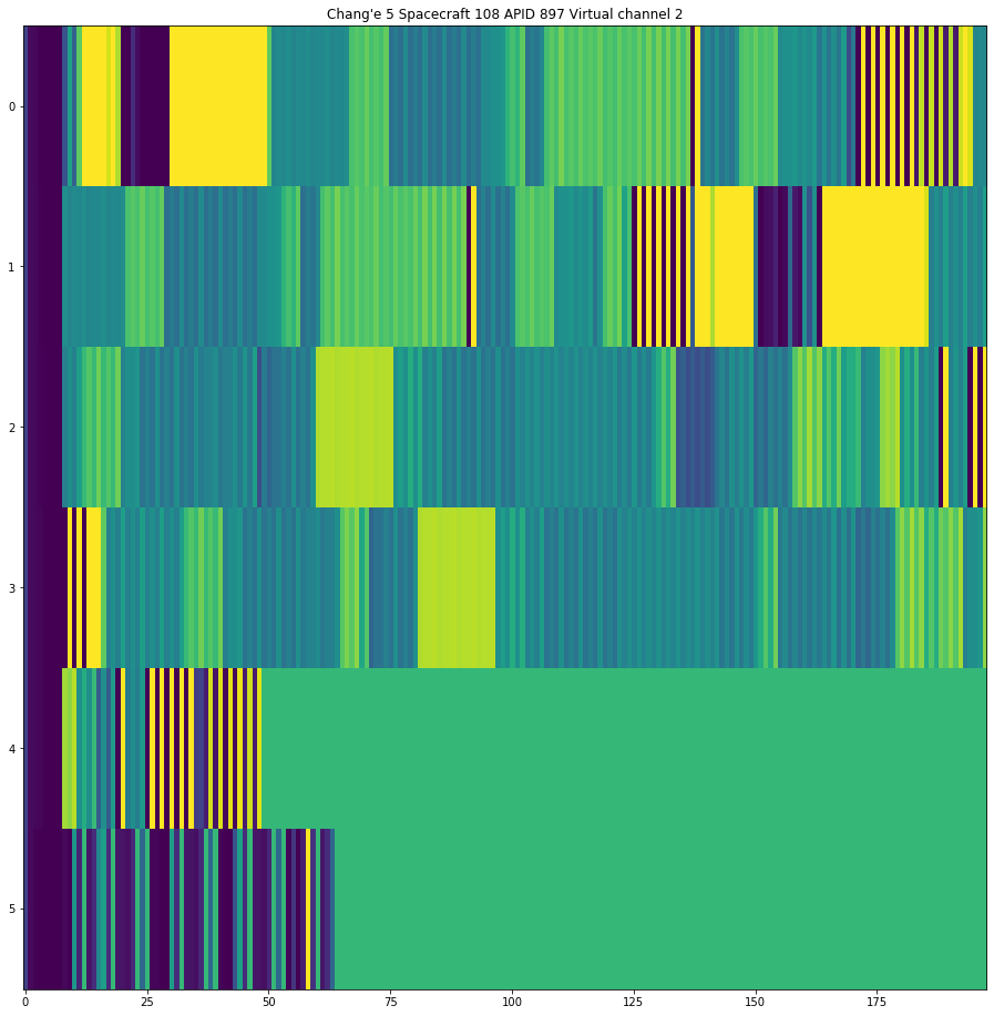
Each of the AOS frames in Virtual Channel 2 is completely filled up with a Space Packet (but still has an M_PDU header, as in Virtual Channel 2). Exactly the same Space Packets are sent by both spacecraft (even the packet count field is the same). There are a number of APIDs in use: 130, 131, 141, 142, 168, 897 and 936. Some of the APIDs use padding bytes at the end of the Space Packets, since all the Space Packets have a fixed payload size of 198 bytes.

APID 897 seems to contain exactly the same data as in the recording I analysed in my previous post, plus one extra packet at the end. Other APIDs look more or less similar to this.

I am not sure of what is the purpose of the packets in Virtual Channel 2.

This is all for this post. There are still many interesting things that can be done with these recordings. The study of the polarization and strength of each of the four signals may tell us something about the spacecraft attitude or the characteristics of its antennas. The Doppler data can be used to obtain more information about the LOI-2 manoeuvre. Scott Tilley has been doing a lot of great work regarding Doppler studies and he has already looked at this data.

The LOI-2 burn is also interesting to try to find out what some of the telemetry channels mean. We have a rough idea of what the spacecraft should be doing regarding its attitude and subsystems, and we can see important changes in many of the values. By plotting some of the fields it might became easier to guess what they represent.

I am not sure how much of this I will be able to do during the next few weeks, but as I said above, all the data will be available in a few days so that anyone can do their own research.

The study of the telemetry in this post has shown that before the separation, which happened several hours after the observation, all the four signals acted pretty much like a single spacecraft, even though the AOS frames used two different spacecraft IDs. The data was completely shared between all the signals. It will be interesting to study how the telemetry data looks like after the spacecraft have separated, as then they can no longer share the data. Maybe some of the APIDs correspond to the systems from one spacecraft and some others correspond the other spacecraft, and so we might see that in each of the spacecraft’s signals the APIDs of the other spacecraft stop being transmitted.