Measuring the ED4YAE 10GHz beacon

Last week, the 10GHz beacon ED4YAE on Alto del León was installed again after having been off the air for quite some time (I think a couple of years). The beacon uses a 10MHz OCXO and a 500mW power amplifier, and transmits CW on 10368.862MHz. The message transmitted by the beacon is DE ED4YAE ED4YAE ED4YAE IN70WR30HX, followed by a 5.8 second long tone.

On 2019-08-31, I went to the countryside just outside my city, Tres Cantos, to receive the beacon and do some measurements. The measurements were done around 10:00 UTC from locator IN80DO68TW. The receiving equipment was a 60cm offset dish from diesl.es, an Avenger Ku band LNB, and a LimeSDR USB. Everything was locked to a 10MHz GPSDO. The dish was placed on a camera tripod at a height of approximately 1.5 metres above the ground.

In this post I show the results of my measurements.

The figure below shows my portable setup. Note the GPS magnetic antenna placed on the roof of the car.

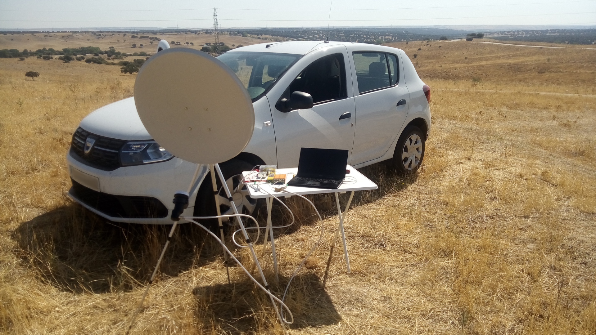
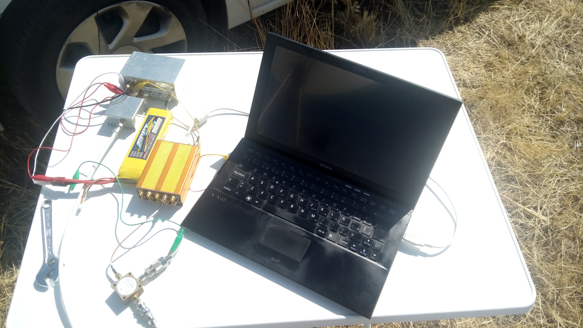
The equipment used was a LimeSDR USB, a DF9NP 10MHz GPSDO connected to the LimeSDR and to a DF9NP 27MHz PLL (used to reference the LNB), a LiPo battery, and a laptop computer running Linrad and GNU Radio.

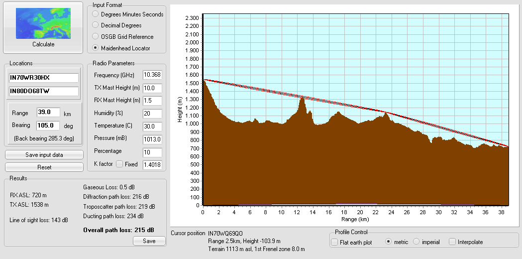
The figure below shows the propagation path from ED4YAE to my station, computed in the SRTM Path Profile software from Mike Willis G0MJW. As you can see, the line of sight path is blocked and the signal refracts on the crest of Sierra de Hoyo de Manzanares midway. This makes it a rather interesting path from the point of view of propagation studies.

Below you can see the view from the top of the dish looking towards ED4YAE. Sierra de Hoyo de Manzanares is visible in the horizon. Behind it, but not visible, is Sierra de Guadarrama, where ED4YAE is located.

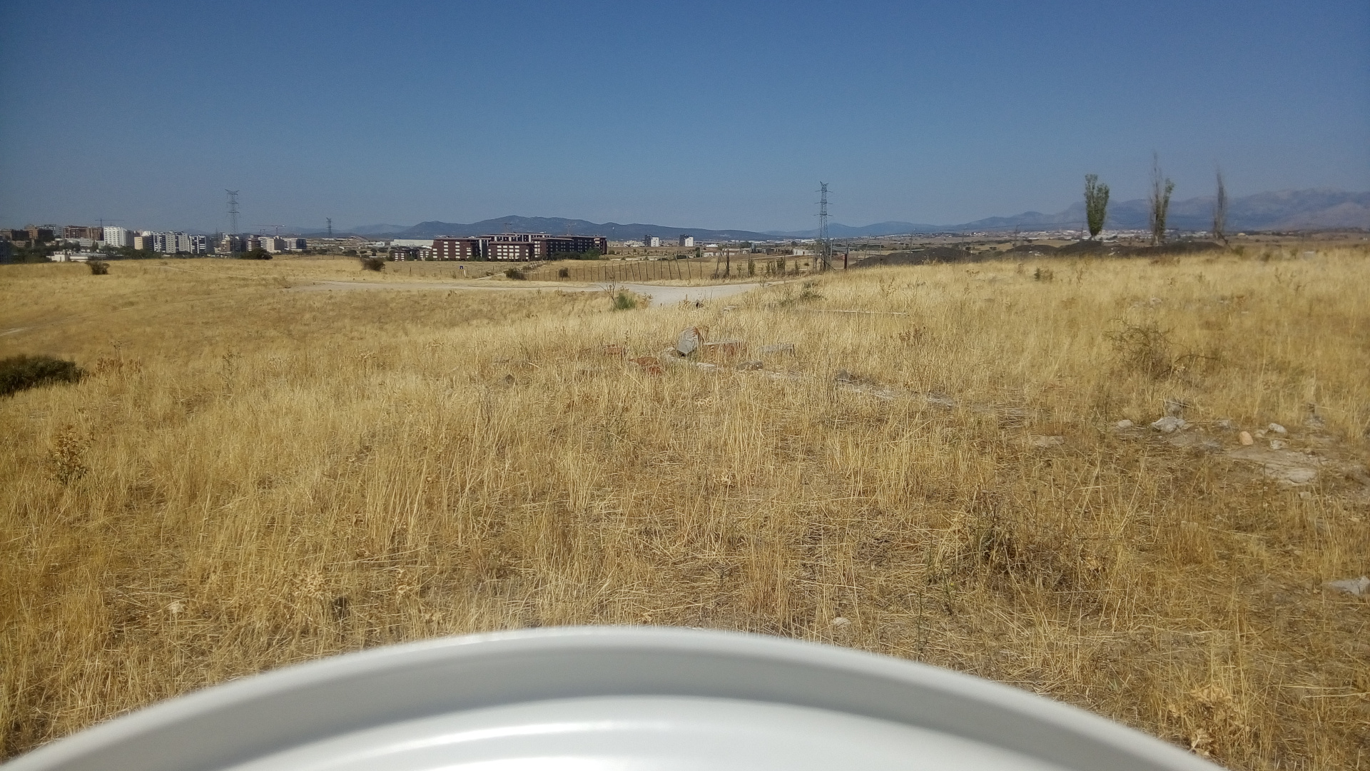
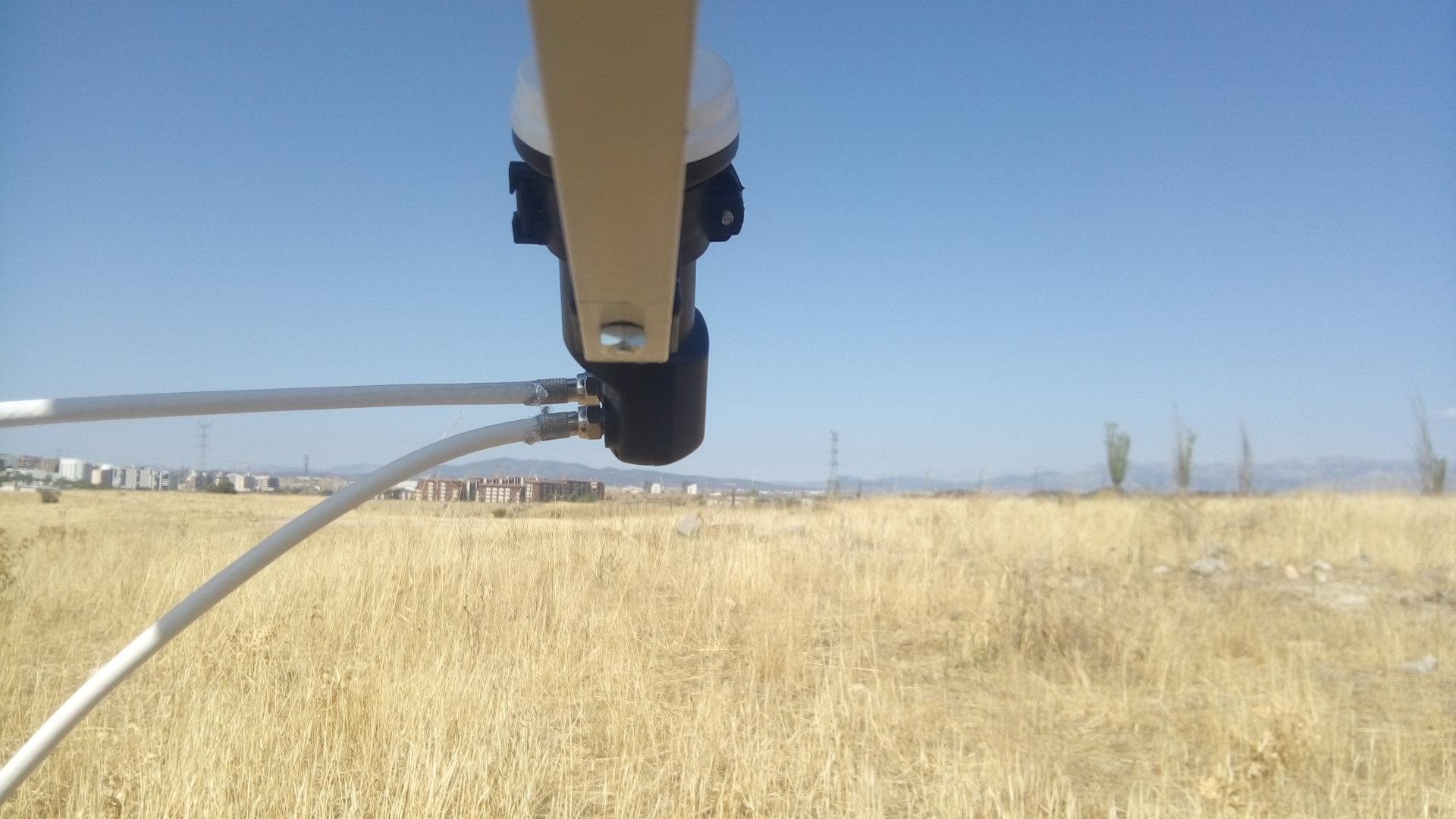
Viewing from the LNB, we see more accurately where the dish is pointing. There are two tall white buildings, one of which might be on the way towards the beacon (click on the image to view it in full size).

I recorded the signal of the beacon for several minutes in order to perform measurements later. The first measurement I have done is a frequency measurement. The beacon frequency is 10368861841 +/-5Hz, where the error accounts for the frequency instability. This is only 159Hz lower than the published frequency. It will be interesting to see how the frequency evolves with oscillator aging.

Next, I have studied the propagation path. It can be modeled as a Rician fading channel, with a a strong “line-of-sight” component and several weaker scattered paths. The Rician model depends on two parameters, \(K\), which gives the power ratio between the direct signal and the scattered signals, and \(\Omega\), which gives the total received signal power (including both the direct and scattered signals).

The estimation of the Rician channel parameters has been done separately on each of the beacon long tones by using the Koay inversion technique. The computations have been done in this Jupyter notebook. The figure below shows the evolution of the channel parameters, expressed in dB’s.

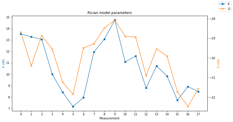
We can see that there is some noticeable channel variation over the 12 minutes that the recording spans. The parameter \(K\) changes by up to 8dB, and \(\Omega\) changes by up to 5dB. Even so, the \(K\) is always above 7dB, so the direct signal is predominant.

The next step is to measure the coherence time of the channel. This indicates how fast the channel characteristics change. This is done both in the complex (amplitude and phase) domain and in the amplitude domain.

The first plot shows the normalized self-correlation of the complex baseband signal for each of the measurements (each measurement corresponds to one of the beacon long tones). A loss in self-correlation is mainly caused by a change of phase of 180º, which causes signal cancellation when integrating coherently (note that the frequency of the signal doesn’t affect the self-correlation as long as it is stable).

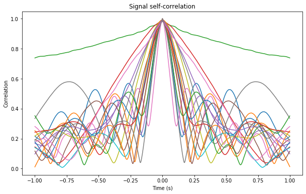
Except for three anomalous measurements where the coherence time is larger (on one of them it is really large, larger than one second), for most of the measurements the coherence time is between 100 and 200ms. Note that the analysis in the complex domain is affected by frequency instabilities in the receiver and the transmitter, as well as small variations in the propagation delay. To determine whether this coherence time is due to the transmitter and receiver or to the propagation path, the same transmitter and receiver should be measured over a short line-of-sight path.

The next figure shows the normalized self-correlation of the amplitude noise. This means that the amplitude of the signal is taken, the mean is removed, and the self-correlation is computed. In a certain sense, this self-correlation describes how fast the channel fading is changing. For a channel that changes fast, the self-correlation will drop down to zero quickly.

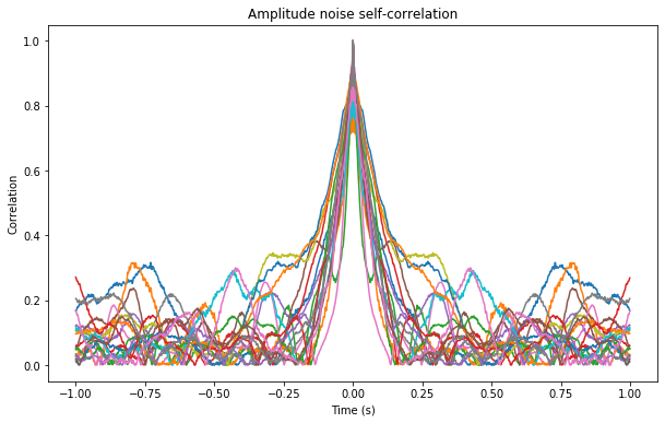
Again, we see coherence times on the order of 100 to 200ms. This analysis in the amplitude domain is not affected by the frequency instabilities of the transmitter and receiver.

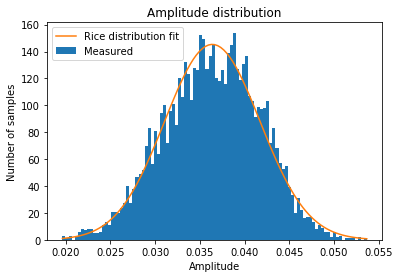
We also examine how good is the fit of the Rician model estimated above to the amplitude measurements. The figure below shows the typical case, in which the fit is good.

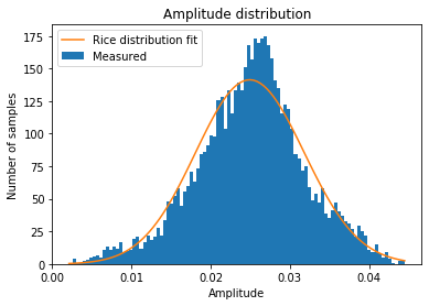
There are a few measurements where the Rician fit is not so good, such as the one showed below. The plots corresponding to all the measurements can be seen in the Jupyter notebook.

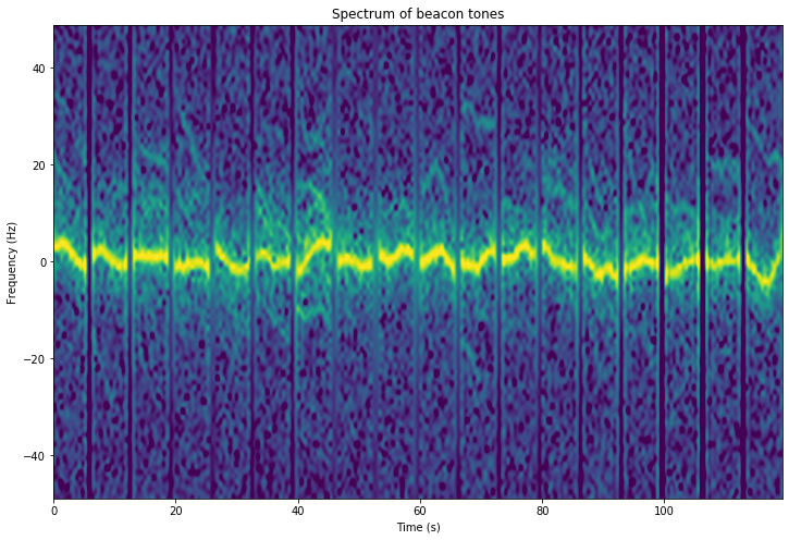
Now we turn to the analysis of the spectrum of the signal. The figure below shows the spectrum of each of the beacon tones. The frequency instability is apparent. There are also some reflections with Dopplers up to 30Hz, which corresponds to 1m/s approximately. The origin of these reflections is unknown.

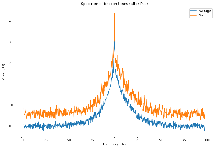
To compensate for the frequency drift of the signal, it is possible to run the signal through a PLL with a bandwidth of 1Hz and then generate the corresponding spectrum. This is shown below.

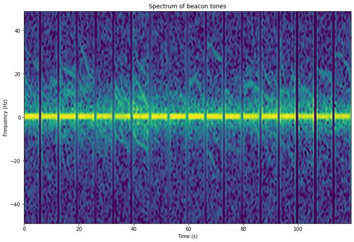
The reflections are now more easily visible and it is apparent that they have a decreasing frequency with a similar slope. This is not surprising. A target moving with constant speed on a bistatic radar will always have decreasing Doppler.

There is also a “diffuse haze” that may be caused by transmitter phase noise, by receiver reciprocal mixing, or by the propagation path. Once again, this test should also be done over a short line-of-sight-path to quantify the phase noise effects due to the transmitter and receiver.

The figure below, which shows the spectrum of the beacon tones after being passed by the PLL, shows the characteristics of this “diffuse haze”.