I have spoken about the Galileo incident that occurred in July in several posts already: here I took a look at the navigation message during the outage, here I used MGEX navigation RINEX files to look at the navigation message as the system was recovering, and here I did the same kind of study for the days preceding the outage. Other people, such as the NavSAS group from Politecnico di Torino, and Octavian Andrei from the Finnish Geospatial Research Institute, have made similar studies by looking at the \(\mathrm{IOD}_{\mathrm{nav}}\), data validity and health bits of the navigation message.
However, I haven’t seen any study about the quality of the ephemerides that were broadcast on the days surrounding the outage. The driving force of the studies has been whether the ephemerides were being updated or not, without taking care to check if the ephemerides that were broadcast were any good at all.
The NavSAS group commented seeing position errors of several hundreds of metres during the outage when using the broadcast ephemerides. That is to be expected, as the ephemerides were already many hours old (and indeed many receivers refused to use them, considering them expired). Here I will look at whether the ephemerides were valid (i.e., described the satellite orbit and clock accurately) in their time interval of applicability.
This post is an in-depth look written for a reader with a good GNSS background.
Approach and software used
The main idea of this study is to compare the satellite orbits and clocks computed with the broadcast ephemerides versus the orbits and clocks computed with precise SP3 files. The broadcast ephemerides are obtained from the IGS BRDC broadcast ephemerides navigation RINEX files from IGS MGEX, as in my previous posts. These files are believed to be representative of the navigation message that was broadcast by the satellites. The SP3 files are obtained from the CNES/CLS final solution, which give satellite orbits and clocks at 15 minutes intervals.
It is common understanding that the Galileo outage affected only the ephemerides, and not the navigation signals. Therefore, the SP3 files should be unaffected by the outage, as they are generated from observations of the navigation signals. We are only concerned with detecting large errors in the broadcast ephemerides, such as orbit errors of several metres or clock errors of several nanoseconds. Thus, SP3 files are perfectly accurate for this goal and it is not necessary to use CLK files with high rate satellite clock products. Hence, the SP3 files are taken as a ground truth description of the satellite orbits and clocks.
To compute the satellite orbits and clocks from the RINEX and SP3 files I have used RTKLIB. I am using version 2.4.3 b33, with some additional modifications described later. I have made a simple C program called compute_satpos that uses RTKLIB to load a RINEX and SP3 file, and computes the orbit and clock of each of the Galileo satellites at one minute spacing using both the broadcast ephemerides from the RINEX and the SP3 file. The results are stored in a binary file that can be read later in a Jupyter notebook for plotting and analysis.
Antenna phase centre versus satellite centre of mass
There is an important technical detail regarding the comparison of broadcast ephemerides and SP3 files. The broadcast ephemerides describe the position of the antenna phase centre, while the SP3 files describe the position of the centre of mass of the satellite. To compare both it is necessary to know the offset of the antenna phase centre with respect to the centre of mass, and the attitude of the satellite. The offset is usually stored in an ANTEX file.
The ANTEX file convention uses a simple model for the satellite attitude that allows to define a satellite-fixed frame of reference in the following way:
- The z-axis points toward the geocenter
- The y-axis (rotation axis of the solar panels) corresponds to the cross product of the z-axis with the vector from the satellite to the Sun
- The x-axis completes the right-handed system
The vector from the centre of mass to the antenna phase centre is described using this frame of reference. Therefore, knowledge of the satellite and Sun positions in ECEF coordinates, together with the information in the ANTEX file, are enough to compute the vector joining the centre of mass and the antenna phase centre in ECEF coordinates.
RTKLIB has the function satantoff() to compute the offset using this algorithm and the information loaded up from an ANTEX file using the function readpcv(). The function satantoff() is automatically called when computing the satellite orbit and clock using satpos(), so that as long as an appropriate ANTEX has been loaded, the antenna phase centre instead of the centre of mass is returned.
The problem is that Galileo has a more sophisticated way of dealing with the offset between the antenna phase centre and the satellite centre of mass. The approach is described in the Galileo Satellite Metadata webpage.
First, a reference frame is defined for the satellite. The axes of this frame correspond to the axes used by the ANTEX file (except for a change of signs in the x- and y- axes), but the origin of the frame is a well defined physical point in the satellite rather than the satellite centre of mass. The motivation for the definition of the reference frame is that the reference frame is fixed with respect to the satellite body, while the position of the centre of mass will change as fuel gets used. By defining the positions of the objects in the satellite body with respect to the reference frame rather than the centre of mass, we get coordinates that don’t change as fuel is spent. To complicate matters further, the reference frame is different for the IOV and for the FOC satellites, since the structure of the satellite body is quite different.
The current and historical positions of the centres of mass of the satellites, measured in the satellite reference frame, can be found in the International Laser Ranging service, as well as in the Galileo Satellite Metadata page.
In order to define the antenna phase centre position, first an antenna reference point is defined. This is a well defined physical point located close to the antenna groundplane, so that its position with respect to the reference frame can be measured physically and will not change. The location of the antenna reference point with respect to the reference frame for each satellite is given in the Satellite Metadata. All the IOV satellites have the same location, and all the FOC satellites have the same location, since these only depend on the physical structure of the satellite.
For convenience, the antenna reference point position is also listed “with respect to ANTEX reference frame”, which means the offset from the centre of mass in the ANTEX xyz frame described above. Note that these offsets will change as fuel is spent.
Finally, the antenna phase centre offset is the vector from the antenna reference point to the antenna phase centre. This is given both in the “mechanical reference frame” and in the “ANTEX reference frame”, but the only difference is the sign of the x- and y- axes, since the origin of the offset is always the antenna phase centre.
An ANTEX file is provided in the Galileo Satellite Metadata page. It gives antenna phase centres and phase centre variations (direction-dependant corrections). However, the ANTEX file is described with respect to the antenna reference point and not to the centre of mass, as expected by the ANTEX file convention. Therefore, RTKLIB won’t work correctly with this ANTEX file.
Another important ingredient to compute the offset between the antenna phase centre and the centre of mass in ECEF coordinates is the attitude of the satellite. As introduced in the ANTEX file convention, one axis of the spacecraft body always points to the geocenter, so that the antenna boresight points to the Earth surface. The spacecraft is then free to rotate around this axis. How it rotates is referred to as yaw steering law. Since the spacecraft needs to orient its solar panels orthogonal to the solar rays, the yaw steering law often dictates that the axis of rotation of the solar panels should be orthogonal to the vector joining the satellite and the Sun, as described in the ANTEX file convention. This is the yaw steering law that is implemented in RTKLIB.
The Galileo Satellite Metadata webpage describes in detail the yaw steering laws of the satellites, in a seemingly different way for the IOV and FOC spacecrafts. Upon closer inspection, it turns out that the yaw steering law for the IOV and FOC satellites is only different in the degenerate case, when the sun angle \(\beta\) (the angle between the orbital plane and the solar rays) is small. In this case special case, the nominal yaw steering law described in the ANTEX file convention is not followed, as it would imply very fast yaw changes. The steering law under these uncommon circumstances is different from the ANTEX file convention, but the rest of the time both the IOV and FOC satellites follow the nominal steering law.
Therefore, we need not worry much about the steering law. The nominal law implemented in RTKLIB is valid for the Galileo satellites in most cases. However, we need an ANTEX file in a suitable format which lists the offsets between the centre of mass and antenna phase centre, rather than the offsets between the antenna reference point and the antenna phase centre, as the Galileo ANTEX file does.
To this end, I have modified the Galileo ANTEX file by using the information in the Galileo Satellite Metadata webpage. To compute the vector joining the centre of mass and the antenna phase centre, it is enough to add the vector listed as “ARP in ANTEX RF” and the vector listed as “PCO in ANTEX RF”. The resulting ANTEX file can be obtained here.
Using this ANTEX file, RTKLIB can compute the antenna phase centre when using an SP3 file, allowing the comparison of broadcast ephemerides and precise SP3 ephemerides.
As an example, the figure below shows the broadcast ephemeris orbit error (i.e., the difference between the orbit computed with the broadcast ephemerides and with the SP3 file) of the satellite E24 in VNB coordinates. The VNB (velocity-normal-binormal) reference frame, which is common in the study of orbital mechanics, was defined in my Lucky-7 precise orbit determination post, and the code for computing this frame is taken from there.
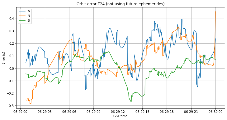
We see that the error in each of the components is smaller than 30cm. Since the offset in the z-axis between the centre of mass and the antenna phase centre is usually between 60 and 80cm (63cm for E24), not correcting for the antenna phase centre offset would cause an error of 60 to 80cm in the binormal component (since the z-axis is almost aligned with the binormal axis, as the orbit is almost circular).
As a final note, no care has been taken in RTKLIB regarding the selection of the frequency band (or bands) for the computation of the antenna phase centre position. Depending on the frequency band, the antenna phase centre offset can change by more than 10cm. The ANTEX file describes the offset for each of the bands E1, E5a, E5b, E6 and E5 (AltBOC). When using an SP3 file with a code or carrier observation in one of these bands, the appropriate antenna phase centre should be computed. If the observation is a linear combination of observations on different bands (for instance, an iononsphere-free combination) it is common to take as phase centre a weighted average of the corresponding antenna phase centres (see the RTKLIB implementation).
When using the broadcast ephemerides, one needs to keep in mind that the I/NAV ephemerides are intended to be used with either E5b, with E1, or with the ionosphere-free combination of E5b and E1, and the F/NAV ephemerides are intended to be used either with E5a, with E1, or with the ionosphere-free combination of E5a and E1. However, the orbit parameters transmitted in the I/NAV and F/NAV ephemerides are the same (or almost the same), so with the broadcast ephemeris model the antenna phase centre position is considered to be the same for all bands. In contrast, the clock \(a_{f0}\) parameters are different in the I/NAV and F/NAV parameters and must be corrected with the appropriate BGD if a single band observation is used, since the difference between the group delays on each band is much larger (something on the order of 50ns, or 15m) than the difference in the phase centre positions.
Interval of applicability of ephemerides
A rather striking fact that I’ve discovered when comparing broadcast ephemeris with precise SP3 files is that it is very important to take into account the interval in which each ephemeris is applicable, understood as the interval in which the error doesn’t grow too large.
It is commonly thought that ephemeris describe an approximation of the orbit about the \(t_{0e}\) timestamp, and they are good for a few hours (4 hours is usually quoted) about this \(t_{0e}\). Therefore, when selecting the best ephemeris to use for a particular timestamp, the one with the nearest \(t_{0e}\) is selected, unless the difference in timestamps is larger than a few hours, in which case it is considered that there is no valid ephemeris for that timestamp. This is what RTKLIB does, as one can see in the function seleph().
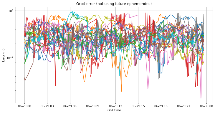
However, this is not completely true, and unexpected problems can appear when using this approach. Let us see an example. In my previous posts about the outage, I used the broadcast ephemerides from 2019-06-29, which was an uneventful day for the Galileo constellation, as some sort of control to check that both my algorithms and the data were correct and no unexpected effects showed up. The figure below shows the orbit error of the broadcast ephemerides for each of the satellites in the constellation during this day.
As we see, E14 and E18, which are the eccentric satellites have errors which sometimes spike up to more than 10m. This is quite large. Upon further inspection we see that the error is largest just after RTKLIB has made a change in the choice of ephemeris. This happens at the midpoint of the \(t_{0e}\)’s of each consecutive pair of ephemerides.
It turns out that Galileo ephemeris are always started to be broadcast by the satellites after their corresponding \(t_{0e}\). I haven’t seen this written in any of the documents, but it is what happens in practice. A look at galmon.eu, a webpage that shows the latest navigation messages transmitted by the GNSS satellites and marks any possible anomaly, reveals that the Galileo ephemeris age is always shown as “x minutes ago”. The same happens for Beidou and GLONASS, so it seems that all these systems start broadcasting the ephemerides after their \(t_{0e}\). In contrast, GPS often shows an age of “in x minutes”, which means that the ephemerides are started to be broadcast before their \(t_{0e}\).
This is important, because a receiver working in real time with the broadcast ephemeris will never use ephemerides which haven’t been broadcast yet. In the case of Galileo, this means that it will never use ephemerides with a \(t_{0e}\) in the future. Therefore, such a receiver will not see the large errors that appear in the figure above.
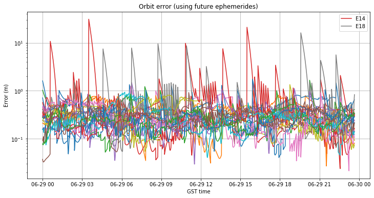
Indeed, I have modified RTKLIB to prevent it from choosing ephemerides with a \(t_{0e}\) in the future. The modified version can be found in my nofutureeph RTKLIB branch. The resulting error with this modified choice of ephemerides is shown below.
The result is strikingly much better than in the case when future ephemerides where chosen. Now the orbit error never exceeds 1m, even for the eccentric satellites E14 and E18. I stress that this goes against the common belief that the choice of ephemeris is not very important as long as the \(t_{0e}\) is not very far off, and that when in doubt one should choose the ephemeris with nearest \(t_{0e}\).
This example teaches a good lesson, but I think it is important to reflect on the matter further. The only official information about when Galileo broadcast ephemeris should or should not be used is the answers to the public consultation about the OS ICD. This document used to be accessible until a couple days ago (indeed I’ve already referenced it in some of my older posts), but now it seems that it’s not available anymore. (Update: the OS SDD is the appropriate replacement for this document).
According to that document, a receiver should always use the latest ephemerides that have been broadcast. If no new ephemeris are broadcast, the ephemerides can be used for up to 3 hours after their \(t_{0e}\). But the moment newer ephemerides are broadcast, the old ones are considered expired and should not be used even if less than 3 hours have passed since their \(t_{0e}\). (Update: the OS SDD also mentions 4 hours in some places).
Thus, I think it is useful to introduce the concept of ephemeris broadcast lifetime. This is the time interval when a particular ephemeris is being broadcast by the satellites. In these terms, the Galileo rules of ephemeris use can be expressed by saying that ephemeris can only be used inside their broadcast lifetime and never more than 3 hours after their \(t_{0e}\).
This raises the natural question of what is the broadcast lifetime, or more precisely, what is the broadcast lifetime in relation to the \(t_{0e}\). We have hinted at this question above when we commented that the broadcast lifetime for Galileo, Beidou and GLONASS seems to start after the \(t_{0e}\), while the broadcast lifetime for GPS seems to start before the \(t_{0e}\).
A comparison between the “transmission time of message” and \(t_{0e}\) fields in the navigation RINEX files show that most of Galileo ephemeris in the RINEX files have been received 740 seconds later than their \(t_{0e}\). Other ephemeris show values larger than 740 seconds, but there is none which was received earlier than this. This seems to indicate that the Galileo ephemeris broadcast lifetime starts 740 seconds (12 minutes and 20 seconds) after the \(t_{0e}\). I haven’t seen this value indicated anywhere in the documentation. This is also surprising, considering that often ephemeris are updated every 10 minutes.
By now it is clear that the ephemerides are designed to be used only during their broadcast lifetime. This is illustrated by the example above. The case in which we don’t use future ephemeris doesn’t completely follow the broadcast lifetime rules (as it starts to use an ephemeris at its \(t_{0e}\) rather than 740 seconds after the \(t_{0e}\)), but gives good results. In contrast, the case in which we use future ephemeris shows the problems that can arise whenever ephemeris are used several tens of minutes away from their broadcast lifetime (more on this will appear in the sequel).
Once that it is clear what is the intended applicability interval for the ephemerides, the natural question is what is the real applicability interval. In other words, how much away from the broadcast lifetime can we use the ephemerides without obtaining a too large error. Another important question is why, meaning what makes the error grow relatively quick outside of the broadcast lifetime to the point that ephemerides are no longer usable.
Again, this is best illustrated with a particular example taken from the control day. The figure below shows the orbit error in VNB coordinates for the satellite E13 (a rather uninteresting and normal satellite) both using the choice of future ephemerides (solid lines) and avoiding the choice of future ephemerides (dashed lines).
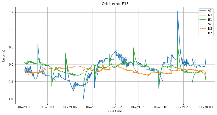
We see that even though the error doesn’t grow to 10m as it happened with the eccentric satellites when we chose future ephemerides, still there are some large spikes that correspond to the future ephemerides. Half of the time the solid and dashed lines coincide, since both are using the same ephemerides. The remaining half of the time they don’t coincide, because the solid line has already changed to the next ephemeris while the dashed line still maintains the old ephemeris. By changing later, the dashed line avoids the large errors.
If we reflect upon this, we can see that there is something that is perhaps not very reasonable. The error grows rather quickly. In the figure above, in some 30 minutes it grows to more than 1 metre. I don’t think that the error in GPS grows as quickly, since often the GPS ephemerides are used more than 1 hour away from their \(t_{0e}\), and the error obtained when doing so is not several metres.
I think it is interesting to look at the moments in the figure above when ephemerides are being refreshed every 10 minutes. These parts look like a zigzag line in the graph due to the frequent changes between different ephemeris. Now, the orbit error might be quite small, but the derivative of the error is large. Only by jumping to a new ephemeris (and producing a discontinuity) the error is maintained small. However, if we use one of these ephemeris one hour away from their \(t_{0e}\), we find that the error has grown very quickly.
This effect is best seen in the figure below, which shows the orbit error for the eccentric satellite E14 when not using future ephemerides. We see that the derivative of the error is very large at the moments when the ephemerides are changed every 10 minutes. Only by jumping to new ephemeris the error is kept small. If we propagate one of these ephemerides much longer than 10 minutes, we get a very large error, which is what happened when using future ephemerides.
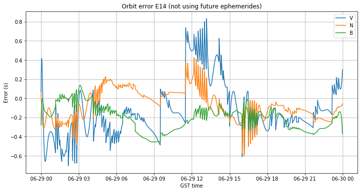
This also seems to explains why ephemerides are sometimes changed every 10 minutes and sometimes not, which was a question in one of my previous posts. The change every 10 minutes is only done when it is necessary to keep the error small because of the error derivative being large. When the derivative of the error is small, such as around 09:00 in the figure above, the same ephemeris can be maintained for more than an hour, since no change is needed to keep the error small.
And now the question is why is the error derivative so large sometimes. Recall that a Keplerian orbit depends on 6 parameters, so to each spacecraft state vector (position and velocity vectors) there corresponds a unique Keplerian orbit that can be considered as the osculating orbit. This is the orbit that the spacecraft would follow if the only force acting upon it was the spherical gravitational force of the central body.
The broadcast ephemerides are based on the Keplerian orbit but include additional perturbations to give a more accurate approximation to the real orbit. These are \(\Delta n\) (a perturbation of mean motion), \(\dot{\Omega}\) and \(\dot{i}\) (the time derivatives of the RAAN and inclination), and harmonic corrections to the anomaly, inclination and orbit radius. Therefore, the broadcast ephemeris model can be considered overdetermined. While for each time there is a single Keplerian orbit that is osculating to the real orbit at that time, the broadcast ephemeris model has many additional perturbation parameters that can be used to obtain a better fit over a time interval. There is much freedom in how to choose these parameters to obtain good results.
I am suspicious that there is perhaps a problem of overfitting with the Galileo ephemerides. By trying to compute the parameters that give the best fit in a certain time interval (probably the broadcast lifetime interval), the model obtained could give a rather poor fit outside of that interval. This is a well known phenomenon that appears in approximation theory. For example, if we try to approximate a continuous function by a polynomial uniformly in some interval, such polynomial will often give a poor fit outside of that interval.
So if I had to guess, I would say that, by trying to improve the broadcast ephemeris fit in some particular interval, too large perturbations to the Keplerian model are chosen. These give a good fit inside said interval, but the error grows quickly, so the fit outside the interval is poor. However, this is probably a topic for a future post.
Control day: 2019-06-29
First we look at the ephemeris error during the control day, June 29, which I chose as an uneventful day for the Galileo constellation. The figures below show the broadcast ephemeris orbit and clock errors when allowing RTKLIB to choose future ephemerides (this has been treated in the previous section). Only the satellites that exceed some predefined error are identified in the legend.

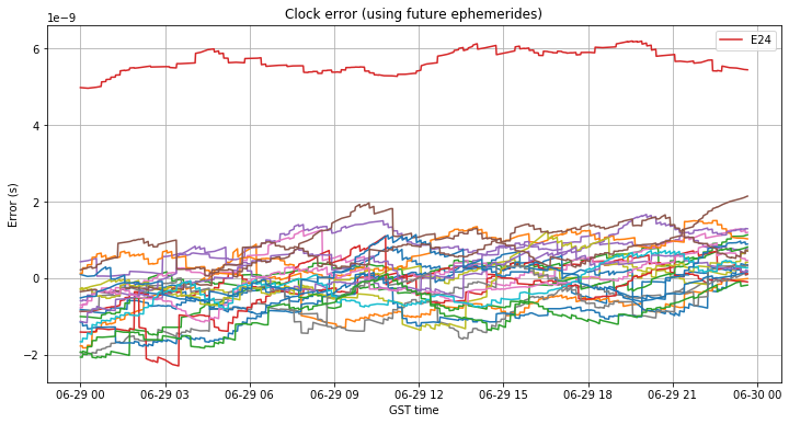
As we have remarked in the previous section, the orbit error stays under 1m except for the eccentric satellites E14 and E18. The clock error of all the satellites is well bounded between -2 and 2 ns, except for E24, which shows a clock error around 6ns. I don’t know what is the cause of this discrepancy, but it is present in all the other days I have analyzed.
If we do not allow RTKLIB to choose future ephemerides, we get the results shown in the figures below.

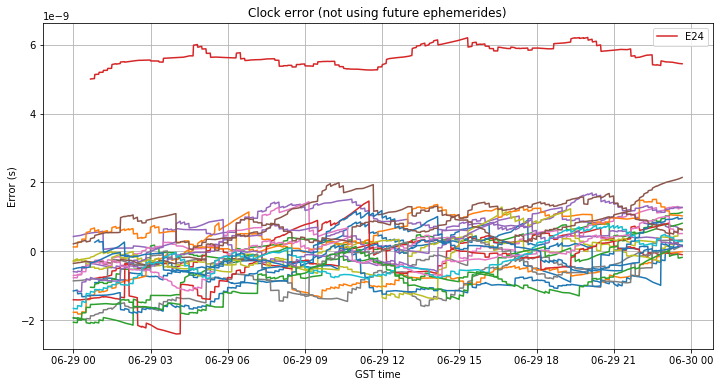
The orbit error has now improved significantly. It is under 1m for all satellites, and usually around 20 to 30cm. The clock error behaves very similarly independently of whether future ephemeris are used or not.
Following the reasoning about the ephemeris broadcast life described in the previous section, the case when future ephemerides are not used will be taken as representative of the broadcast ephemeris quality in all the scenarios.
Now that we know what errors to expect from the broadcast ephemerides during a regular day, we can pass to study the scenarios corresponding to the days before and after the outage.
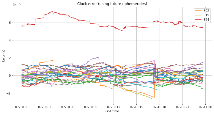
Day before the outage: 2019-07-10
The behaviour of the navigation message on the two days before the outage can be found in this post. The figure below, taken from that post, summarizes the evolution of the \(\mathrm{IOD}_{\mathrm{nav}}\).
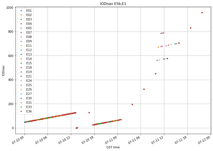
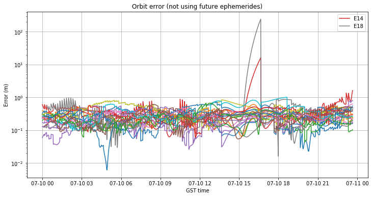
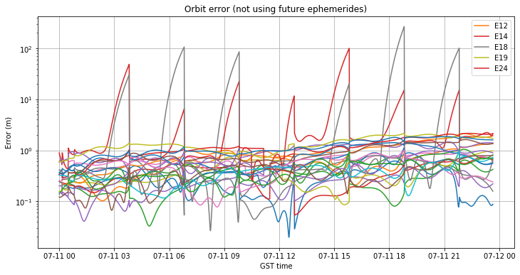
We see that on July 10 there is a long gap in the broadcast ephemerides between approximately 13:40 and 16:40 GST. Ephemerides are broadcast again at 16:40, but after this there are no ephemerides until 17:30.
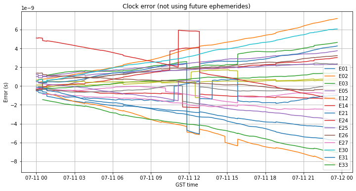
The figures below show the orbit and clock errors when future ephemerides are not used. The gap between 13:40 and 16:40 is apparent. The eccentric satellites E14 and E18 quickly pick up very large orbit errors: more than 10m and 100m respectively. In comparison, the other satellites stay with errors below 1m.
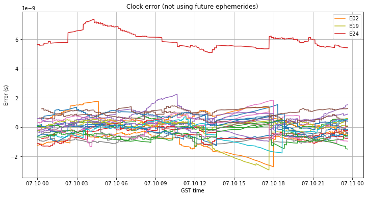
The clock error diverges linearly during the gap. This behaviour is to be expected, since the broadcast ephemeris clock model is usually a linear function (a quadratic function is also supported) but the estimation of the slope \(a_{f1}\) will never be perfect. The divergence is small, so only E02 and E19 exceed 2.5ns of clock error. However, it is interesting that with the ephemerides of 16:40 the clock error isn’t corrected and keeps growing. I believe that this is caused by a problem with the determination of the satellite clocks by the ground segment. This will be more clear with the analysis of the next day.
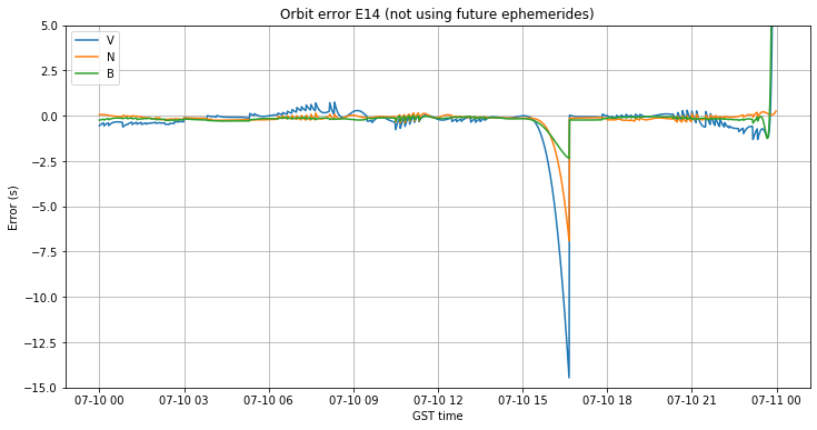
If we plot the orbit error of E14, we see that even though the last set of ephemerides before the gap was at 13:40, the error stays reasonably small until 15:00. Sometime after 15:00 the error grows up very quickly in all the components of the VNB frame. This shows the problems remarked above about the interval of applicability of the broadcast ephemerides, which often seems too small, causing problems like this when no updated ephemerides are broadcast.
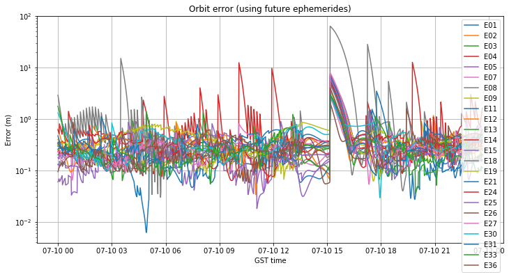
If we allow RTKLIB to use future ephemerides, we get the orbit and clock errors shown in the figures below. This time all the satellites get large orbit errors at 15:10, often reaching up to 8m. The reason is that RTKLIB is using the ephemerides from 16:40 rather than those from 13:40. This gives a good example of why the usual rule of choosing the broadcast ephemerides with nearest \(t_{0e}\) may not be a good idea for Galileo. Propagating ephemerides backwards gives larger errors than propagating forwards.
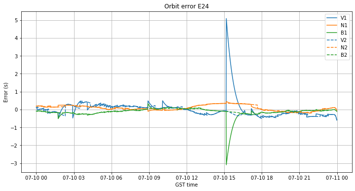
For an more detailed example of this effect, the figure below shows the orbit error of E24 with future ephemerides (solid line) and no future ephemerides (dashed line). We see that between 15:10 and 16:00, when using the future ephemerides, the ephemeris from 16:40 is chosen, causing a large error. In contrast, when using no future ephemerides, the ephemeris from 13:40 is chosen and the error is kept small. I think this kind of examples support my idea that Galileo ephemerides are overfitted in a certain sense.
In summary, on July 10 there was a 3 hour gap in ephemerides between 13:40 and 16:40. The impact to the system performance was small but noticeable for the non-eccentric satellites and receivers using the broadcast lifetime rule. However, there was a large degradation in performance for the eccentric satellites and for postprocessing using the ephemerides with nearest \(t_{0e}\).
Outage day: 2019-07-11
In July 11 there were a few sets of ephemerides broadcast at the beginning of the day, but at 00:50 the broadcast changed to every 3 hours, except for some satellites that transmitted a few ephemerides outside of this schedule (see more details in the previous post).
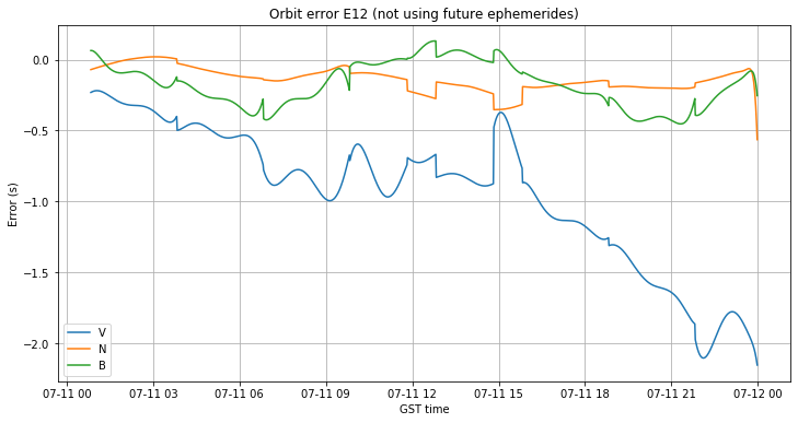
The orbit and clock errors not using future ephemerides are shown in the two figures below. Regarding the orbit error, we see the same problems on the eccentric E14 and E18 as on July 10, caused by the large 3 hours gaps in the ephemerides. We also note a slow but noticeable tendency of the orbit error of all the other satellites to increase throughout the day. By the end of the day, E12, E19 and E24 already have picked up more than 2m of orbit error.
Regarding the clock error, we see that it grows linearly for all the satellites. There are some strange jumps around 12:00. These seem to correspond to satellites transmitting out of the 3 hour schedule, since there is always a first jump that is not aligned with the 3 hour schedule and only happens for a single satellite, and then a second jump coincident with the 3 hour schedule, where all the satellites that jumped go back to the previous clock error trend. I have no clue about what could cause these jumps, but they are certainly interesting.
Other than the jumps, it seems that the clock model is not being updated regardless of the fact that new ephemerides are broadcast every 3 hours. It seems that the determination of satellite clocks by the ground segment was not working at all. By the end of the day some of the satellites have already picked up to 8ns (or 2.4m) of clock error.
The figure below shows the orbit error of E12 in VNB coordinates. This was one of the satellites whose error grew largest. We see that the error grows mostly in the V component. This is usual in orbital mechanics. Every inaccuracy in the orbit model manifests much more in the V component, since errors such as an error in mean motion build up with time, causing an increasing error in mean anomaly.
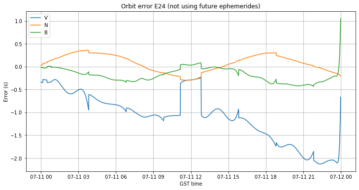
Below we show the orbit error of E24, which is one of the satellites whose clock jumped. There is a jump in the orbit and it is aligned with the clock jump. We also see the error buildup in the V component.
Finally, we show the orbit and clock errors when RTKLIB is allowed to choose future ephemerides. The characteristic problem with using future ephemerides happens now for all the satellites every 3 hours, causing orbit errors of several metres.
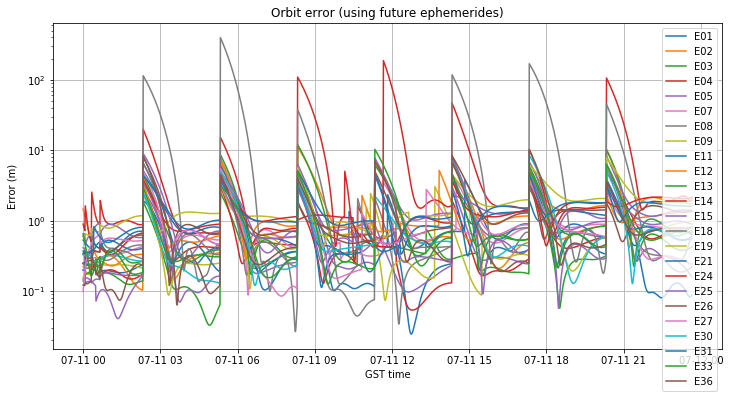
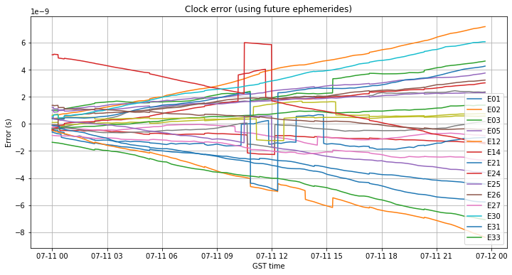
In summary, on July 11 the performance of the system was degraded even for receivers using non-eccentric satellites and the broadcast lifetime rule. By the end of the day, many satellites had grown orbit errors near 1m and clock errors near 5ns. It seems that the clock model of the satellites wasn’t updated throughout the day, letting the clock error grow linearly.
First day of recovery: 2019-07-16
On July 16, most of the satellites started broadcasting updated ephemerides again at 18:50, after having been several days broadcasting the same old set of ephemerides. The remaining satellites joined a few hours later. More details can be seen in this post.
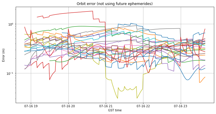
The figures below show the orbit and clock errors when future ephemerides are not used. The orbit error is smaller than 1m for most of the satellites, and perhaps it seems to improve somewhat during the course of the day.
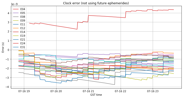
The clock error seems also well controlled, but in comparison to the control day 2019-06-29, it seems that the clock errors of all the satellites are shifted down around 2ns.
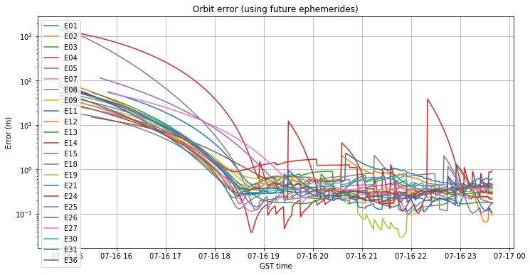
If we let RTKLIB use future ephemerides, it propagates backwards the ephemerides from 18:50 until 14:50. We see that the orbit error grows almost exponentially with time. At three hours of propagation the error is around 10m for most of the satellites, and 100m for the eccentric satellites. At four hours, the error is between 50 and 100m for most of the satellites, and the eccentric satellites reach 1km of error. This shows that, in general, the Galileo broadcast ephemerides cannot be propagated for 3 or 4 hours.
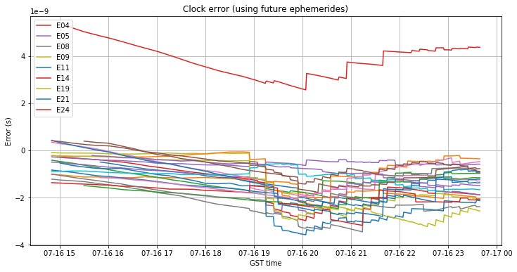
On the other hand, the clock error grows linearly but slowly when propagating the ephemerides backwards. After 4 hours of propagation, the error has perhaps grown 0.25ns, which is completely acceptable.
The figure below shows the growth of the orbit error when propagating backwards the ephemeris of E24. The error grows mainly in the V component, but the error in N and B is also large.
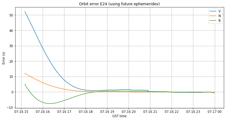
If we don’t allow RTKLIB to use future ephemerides, we get the orbit error shown below instead. It seems that the orbit of E24 was refined during the course of the day. The V error started large and with an increasing trend, but dropped down significantly at 21:00.
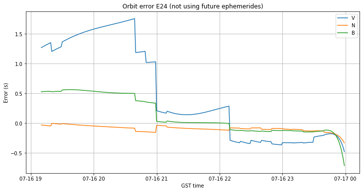
In summary, once that updated ephemerides were broadcast on July 16, the performance of the system was almost back to normal. It seems that there was some slight improvement in the ephemeris quality during the course of the day. However, the first updated ephemerides available shouldn’t be propagated backwards, as this causes significant errors.
Second day of recovery: 2019-07-17
On July 17 the satellites continued broadcasting updated ephemerides normally, and the SISA flag was changed from NAPA to 3.12m at 17:50. Officially, the system was restored at 20:52 according to NAGU 2019027.
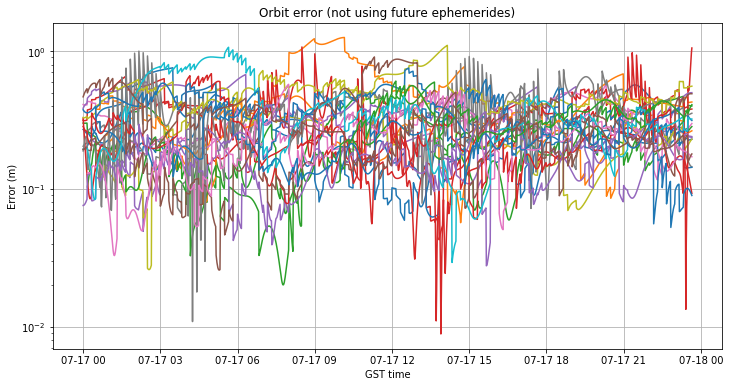
The figure below shows the orbit and clock errors when not using future ephemerides. The orbit error is below 1m for most satellites and looks quite on par with the control day 2019-06-29. Therefore, it seems that the orbit determination is working well again.
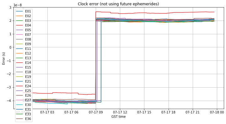
The clock error is much more striking and interesting. Even though we left a rather good clock error of around -1ns at the end of July 16, now it has jumped to -40ns at the beginning of July 17. Around 9:00 it jumps to 20ns. All the satellites seem to jump by the same amount of 60ns, but they don’t jump simultaneously.
In my opinion, this jump of 60ns shouldn’t be read as a jump of the broadcast satellite clock models, but rather a jump of the GST “paper clock”. To be precise, the clock error plot above shows the difference between the broadcast clocks in the RINEX navigation file and the precise clocks in the SP3 file. The broadcast clocks describe the difference between the satellite clocks and the GST paper clock. The SP3 file describes the difference between the satellite clocks and the reference clock that CNES is using to generate its multi-GNSS solution (which is probably tied in one way or another to UTC). Therefore, the jumps in the plot can be produced by jumps in the GST paper clock, in comparison with the CNES reference clock.
In summary, during July 17 the system performance was back to normal except for the GST-UTC offset. It seems that this offset started at -40ns and jumped to 20ns around 9:00.
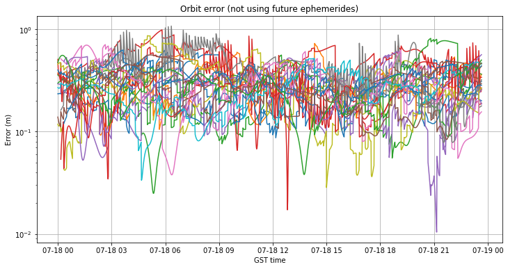
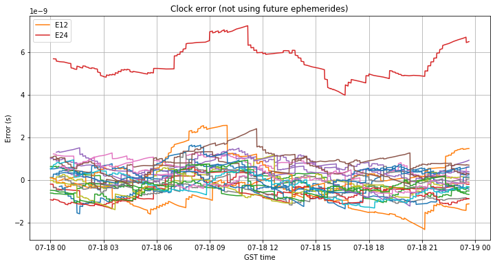
Third day of recovery: 2019-07-18
July 18 wasn’t covered in any of my studies, since the performance of the Galileo system seemed back to normal already on July 17, and the system was deemed to be operational by 20:52 on July 17. However, in view of the fact shown above that the GST-UTC offset was still around 20ns at the end of July 17, I have decided to analyze July 18 to see when the GST-UTC offset was recovered.
The figures below show the orbit and clock errors, without using future ephemerides. The orbit error is below 1m in almost every case. The clock error is back to normal, so it seems that GST was aligned again with UTC at the start of July 18.
Appendix: material
The software used in this post can be found in my galileo-outage collection of Jupyter notebooks. This folder also contains the following:
compute_satpos.cC program to compute the satellite orbits and clocks with RTKLIB using RINEX and SP3 files- The RINEX and SP3 files used in the study
GSAT_2023_ANTEXRF.atxthe ANTEX file describing the satellite antenna phase centre offsets with respect to the centres of mass- The Jupyter notebook used to create the figures shown in this blogpost.
Additionally, two versions of RTKLIB were used:
rtklib_2.4.3, which selects the ephemeris with nearest \(t_{0e}\)nofutureeph, which never selects future ephemeris
extremely interesting article. i was trying to find WHY the time of transmission of the message in Galileo RINEX files is later than toe.
thank you!