Yesterday we had a strong storm in Madrid at around 16:30 UTC. The storm was rather short but intense. Seeing the heavy rain, it occurred to me that I might be able to receive the 10 GHz beacon ED4YAE at Alto del León using my QO-100 groundstation (without moving the antenna).
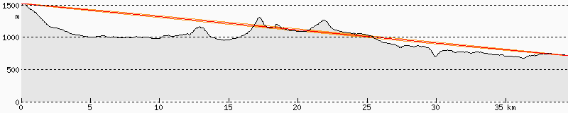
The 10 GHz beacon is 39.4 km away and the direct path to my station is obstructed by some hill in the middle, as shown in the link profile.
In the countryside just outside town it is possible to receive the beacon, probably because it diffracts on the hills. However, it is impossible for me to receive it directly from home, as there are too many tall buildings in the way.
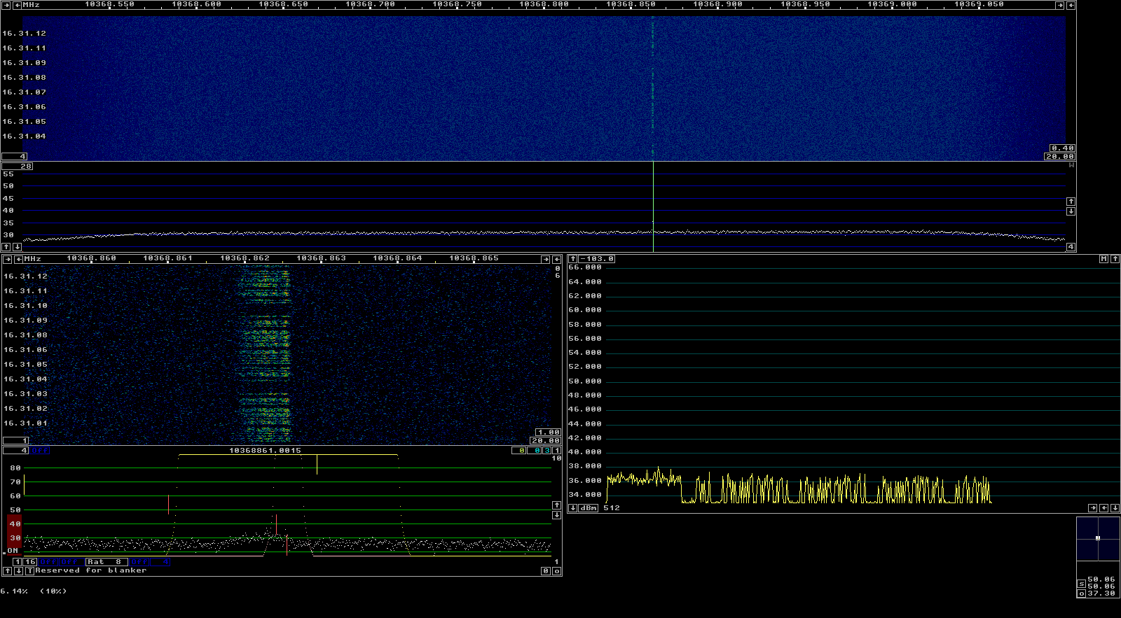
In fact, when I fired up my receiver as the storm raged, I was able to see the beacon signal, with a huge Doppler spread of some 700 Hz (20 m/s). The CW ID of the beacon was easy to copy.
ED4YAE -> EA4GPZ at 10 GHz via rain backscatter
Then I started recording the signal. As the rain got weaker, it started disappearing, until it faded away completely. This post is a short analysis of the scatter geometry and the recording.
Over the last few weeks I have been helping the Allen Telescope Array by calibrating the pointing of some of the recently upgraded antennas using the GNU Radio backend, which consists of two USRP N32x devices that are connected to the IF output of the RFCB downconverter. For this calibration, GPS satellites are used, since they are very bright, cover most of the sky, and have precise ephemerides.
The calibration procedure is described in this memo. Essentially, it involves pointing at a few points that describe a cross in elevation and cross-elevation coordinates and which is centred at the position of the GPS satellite. Power measurements are taken at each of these points and a Gaussian is fitted to compute the pointing error.
The script I am using is based on this script for the CASPER SNAP boards, with a few modifications to use my GNU Radio polarimetric correlator, which uses the USRPs and a software FX correlator that computes the crosscorrelations and autocorrelations of the two polarizations of two antennas. For the pointing calibration, only the autocorrelations are used to measure Stokes I, but all the correlations are saved to disk, which allows later analysis.
In this post I analyse the single-dish polarimetric spectra of the GPS satellites we have observed during some of these calibrations.
A few days ago, the spring eclipse season for Es’hail 2 finished. I’ve been recording the frequency of the NB transponder BPSK beacon almost 24/7 since March 9 for this eclipse season. In the frequency data, we can see that, as the spacecraft enters the Earth shadow, there is a drop in the local oscillator frequency of the transponder. This is caused by a temperature change in the on-board frequency reference. When the satellite exits the Earth shadow again, the local oscillator frequency comes back up again.
The measurement setup I’ve used for this is the same that I used to measure the local oscillator “wiggles” a year ago. It is noteworthy that these wiggles have completely disappeared at some point later in 2020 or in the beginning of 2021. I can’t tell exactly when, since I haven’t been monitoring the beacon frequency (but other people may have been and could know this).
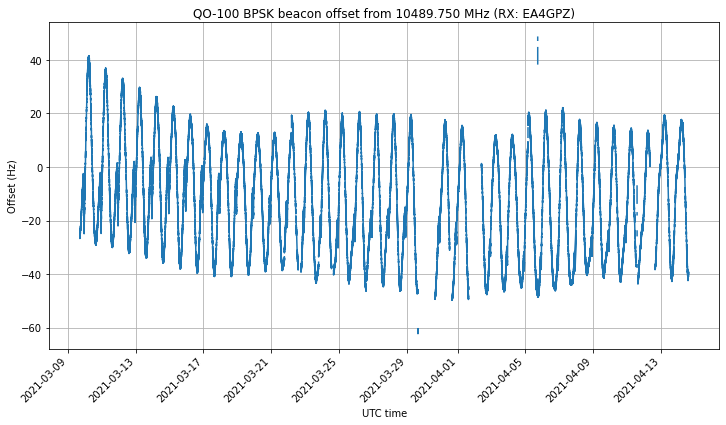
A Costas loop is used to lock to the BPSK beacon frequency and output phase measurements at a rate of 100 Hz. These are later processed in a Jupyter notebook to obtain frequency measurements with an averaging time of 10 seconds. Some very simple flagging of bad data (caused by PLL unlocks) is done by dropping points for which the derivative exceeds a certain threshold. This simple technique still leaves a few bad points undetected, but the main goal of it is to improve the quality of the plots.
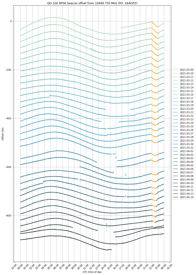
The figure below shows the full time series of frequency measurements. Here we can see the daily sinusoidal Doppler pattern, and long term effects both in the orbit and in the local oscillator frequency.
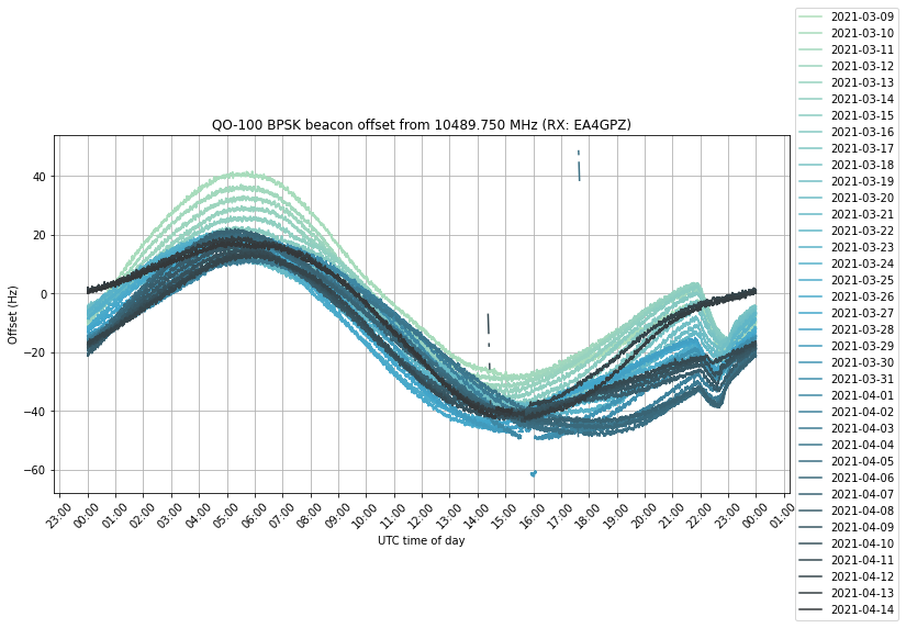
If we plot all the days on top of each other, we get the following. The effect of the eclipse can be clearly seen between 22:00 and 23:00 UTC.
By adding an artificial vertical offset to each of the traces, we can prevent them from lying on top of each other. We have coloured in orange the measurements taken when the satellite was in eclipse. The eclipse can be seen getting shorter towards mid-April and eventually disappearing.
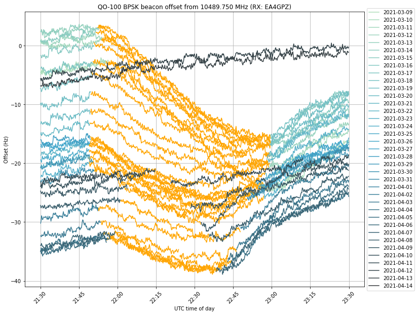
We see that the frequency drop starts exactly as soon as the eclipse starts. In many days, the drop ends at the same time as the eclipse, but in other days the drop ends earlier and we can see that the orange curve starts to increase again near the end of the eclipse. This can be seen better in the next figure, which shows a zoom to the time interval when the eclipse happens, and doesn’t apply a vertical offset to each trace. I don’t have an explanation for this increase in frequency before the end of the eclipse.
The plots in this post have been done in this Jupyter notebook. The frequency measurements have been stored in this netCDF4 file, which can be loaded with xarray.
Back in 2019, I took advantage of the autumn sun outage season of Es’hail 2 to make some observations as the sun passed in front of the fixed 1.2 metre offset dish I have to receive the QO-100 transponders. Using the data from those observations, I estimated the gain of the dish and the system noise. A few weeks ago, I have repeated this kind of measurements in the spring sun outage season this year. This post is a summary of the results.
In the weekend experiments that we are doing with the GNU Radio community at Allen Telescope Array we usually have access to some three antennas from the array, since the rest are usually busy doing science (perhaps hunting FRBs). This is more than enough for most of the experiments we do. In fact, we only have two N32x USRPs, so typically we can only use two antennas simultaneously.
However, for doing interferometry, and specially for imaging, the more antennas the better, since the number of baselines scales with the square of the number of antennas. To allow us to do some interferometric imaging experiments that are not possible with the few antennas we normally use, we arranged with the telescope staff to have a day where we could access a larger number of antennas.
After preparing the observations and our software so that everything would run as smoothly as possible, on 2021-02-21 we had a 18 hour slot where we had access to 12 antennas. The sources we observed where Cassiopeia A and Cygnus A, as well as several compact calibrators. After some calibration and imaging work in CASA, we have produced good images of these two sources.
Many thanks to all the telescope staff, specially to Wael Farah, for their help in planning together with us this experiment and getting everything ready. Also thanks to the GNU Radio team at ATA, specially Paul Boven, with whom I’ve worked side by side for this project.
This post is a long report of the experiment set up, the software stack, and the results. All the data and software is linked below.
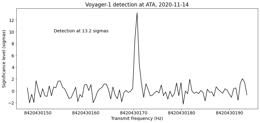
This post has been delayed by several months, as some other things (like Chang’e 5) kept getting in the way. As part of the GNU Radio activities in Allen Telescope Array, on 14 November 2020 we tried to detect the X-band signal of Voyager-1, which at that time was at a distance of 151.72 au (22697 millions of km) from Earth. After analysing the recorded IQ data to carefully correct for Doppler and stack up all the signal power, I published in Twitter the news that the signal could clearly be seen in some of the recordings.
Since then, I have been intending to write a post explaining in detail the signal processing and publishing the recorded data. I must add that detecting Voyager-1 with ATA was a significant feat. Since November, we have attempted to detect Voyager-1 again on another occasion, using the same signal processing pipeline, without any luck. Since in the optimal conditions the signal is already very weak, it has to be ensured that all the equipment is working properly. Problems are difficult to debug, because any issue will typically impede successful detection, without giving an indication of what went wrong.
I have published the IQ recordings of this observation in the following datasets in Zenodo:
Bill Gray, from Project Pluto is doing a great job trying to estimate the orbit of Chang’e 5 as it travels to somewhere around the Sun-Earth L1 Lagrange point (see my previous post). He is using RF pointing data from Amateur observers and the Allen Telescope Array, since the low elongation and the distance of the spacecraft have made it impossible to observe it optically.
For this task, the pointing data I am obtaining with my observations on Allen Telescope Array as part of the activities of the GNU Radio community there is quite valuable, since the 6.1 metre dishes give more accurate pointing measurements than the smaller dishes of Amateurs. The pointing data from ATA should be accurate to within 0.1 or 0.2 degrees.
To try to get more accurate data for Bill, last weekend I decided to do a recording with two dishes from the array, with the goal of using interferometry to obtain a much more precise pointing solution that what can be achieved with a single dish. This post is a report of the processing of the interferometric data.
In my previous post, I talked about an observation of Chang’e 5 made with Allen Telescope Array last Sunday, 2020-11-29. I still need to write the report corresponding to the observation from Saturday 2020-11-28. However, before doing so, I thought it would be interesting to look at the polarization of each of the signals in these recordings. As I already advanced, the polarization is not perfect RHCP, but rather elliptical and time varying.
In fact, it seems likely that most of the antennas of Chang’e 5 are not steerable antennas, but rather, patch-like medium-gain or low-gain antennas. These are circularly-polarized only when seen from the front. They are linearly polarized when seen from a side.
Therefore, by studying the polarization of the Chang’e X-band signals, we can try to learn more about the spacecraft’s attitude and its antennas.
If you follow me on Twitter you’ll probably have seem that lately I’m quite busy with the Chang’e 5 mission, doing observations with Allen Telescope Array as part of the GNU Radio activities there and also following what other people such as Scott Tilley VE7TIL, Paul Marsh M0EYT, r00t.cz, Edgar Kaiser DF2MZ, USA Satcom, and even AMSAT-DL at Bochum are doing with their own observations. I have now a considerable backlog of posts to write, recordings to share and data to process. Hopefully I’ll be able to keep a steady stream of information coming out.
In this post I study the observation I did with Allen Telescope Array last Sunday 2019-11-29. During the observation, I was tweeting live the most interesting events. The observation is approximately 3 hours long and contains the LOI-2 (lunar orbit injection) manoeuvre near its end. LOI-2 was a burn that circularized the elliptical lunar orbit into an orbit with a height of approximately 207km over the lunar surface.
Following my polarimetry experiments at Allen Telescope Array, on October 31 I did a polarimetric observation of the quasar 3C286 with two dishes from the array to use as a test-bed for polarimetric calibration. 3C286 is a bright, compact, polarized source, with a fractional polarization intensity of around 10% and a polarization angle of 33º over a wide range of frequencies, so it makes an ideal source for polarization calibration. It is the primary polarization calibrator for VLA. The observation duration was slightly more than 2 hours, and it was done around the transit of the source, so the parallactic angle coverage is large (around 90º).
My initial idea was to use this observation to perform a “single dish” polarization calibration of each of the dishes by separate (since the math is somewhat simpler) and then perform an interferometric polarization calibration. However, after initial examination of the data, the SNR doesn’t seem large enough to do a “single dish” calibration. The polarized signal from 3C286 is rather weak and is swamped by noise from other sources in the field and from the receiver, and also by gain variations in the receive chain.
On the contrary, the interferometric calibration has worked well, since correlating the signals from the antennas allows us to discard the uncorrelated receiver noise and to phase on the target and discard other signals from the field, by means of Earth rotation aperture synthesis.
In this post I give my analysis and results of the observation. I have done an ad hoc calibration in Python to determine the polarization leakage and measure the polarization degree and angle of the source, and also a full polarimetric calibration in CASA to compare my calibration with one obtained with professional software.