In the weekend experiments that we are doing with the GNU Radio community at Allen Telescope Array we usually have access to some three antennas from the array, since the rest are usually busy doing science (perhaps hunting FRBs). This is more than enough for most of the experiments we do. In fact, we only have two N32x USRPs, so typically we can only use two antennas simultaneously.
However, for doing interferometry, and specially for imaging, the more antennas the better, since the number of baselines scales with the square of the number of antennas. To allow us to do some interferometric imaging experiments that are not possible with the few antennas we normally use, we arranged with the telescope staff to have a day where we could access a larger number of antennas.
After preparing the observations and our software so that everything would run as smoothly as possible, on 2021-02-21 we had a 18 hour slot where we had access to 12 antennas. The sources we observed where Cassiopeia A and Cygnus A, as well as several compact calibrators. After some calibration and imaging work in CASA, we have produced good images of these two sources.
Many thanks to all the telescope staff, specially to Wael Farah, for their help in planning together with us this experiment and getting everything ready. Also thanks to the GNU Radio team at ATA, specially Paul Boven, with whom I’ve worked side by side for this project.
This post is a long report of the experiment set up, the software stack, and the results. All the data and software is linked below.
Observation set up
The set of 12 antennas that were available to us during this experiment were 1a, 1c, 1f, 1h, 1k, 2a, 2b, 2h, 3c, 4g, 4j, and 5c. However, we decided to discard 3c, since it was having some serious performance problems above 3 or 4 GHz. The cause of these problems was found later: the pointing calibration of this antenna was off, so the target was out of the dish beam for the higher frequencies.
The antennas can be seen in the map below, which also indicates which antennas have the newer cryogenic feeds donated by Franklin Antonio. The longer baselines are a bit over 300 metres.

The choice of the science targets to observe was mainly led by Paul, inspired by this paper about observations of Cassiopeia A, Cygnus A, Taurus A, and Virgo A at 50 MHz with LOFAR. Since this was our first imaging experiment with ATA, we wanted something that was easy to image. This means a bright source that was extended enough to resolve with our 300 metre baselines. Trying to get ideas from VLA is not so good because it has much more sensitivity and resolution than the ATA. Thus, we decided to use Cygnus A as our primary science target and Cassiopeia A as a secondary science target.
The antenna ECEF coordinates were obtained by Mike Piscopo, after managing to make sense of the local-horizon coordinates used by the ATAcontrol Python library. We had validated that a few baselines from these coordinates were pretty close to the baselines we had solved from scratch by doing long observations of compact sources. However we hadn’t validated most of the antenna positions, since we had never used those antennas before the experiment.
We decided to use a frequency of 4.9 GHz for the observations. This frequency would be high enough to resolve well the two components of Cygnus A. We didn’t want to risk going higher in frequency, since the sources would have less flux density (specially the calibrators, which are already much weaker than the science targets) and the baseline errors would be magnified.
There is something unique about the way we do these interferometry observations with the USRPs. A usual interferometer can digitize the signals from all the antennas simultaneously, so it continuously produces correlations for all the baselines. Having two USRPs, we can only digitize the signals from two antennas simultaneously, so we can only obtain correlations for one baseline at a time. Moreover, the set of antennas that can be connected to each USRP was fixed as follows:
- USRP1: 1a, 1c, 2a, 4g, 4j
- USRP2: 1f, 1h, 1k, 2b, 2h, (3c), 5c
This means that we can’t form all the possible 66 baselines between our set of 12 antennas (55 baselines if we discard 3c). We can only form baselines picking one of the USRP1 antennas and one of the USRP2 antennas, which gives us 35 baselines (30 baselines if we discard 3c).
The reason for this limitation is the way that the switch matrix that connects the RFCB to the USRPs is cabled. This is pretty much the best we can do with the equipment at ATA. It would be too much to ask for a switch that can send any antenna to any USRP.
Being limited to observing one baseline at a time comes with some challenges. Even with only 30 baselines, iterating through all the baselines is slow (for instance, with one minute scans, half an hour is spent to go through all the baselines). Once we started planning things, we realize that there are two difficulties:
- Since the calibrators are much weaker than the science targets, the calibrator scans need to be longer. Thus, we risk spending a lot of time observing the calibrator instead of gathering useful visibility for the science target.
- Since going over all the baselines takes so long, it is tempting to plan revisits to a calibrator only after several hours. However this can be risky if the complex gains change faster than the revisit time.
To solve the first problem we noticed that for a successful complex gain calibration we don’t need to go through all the 30 baselines. In fact, it is enough to pick one antenna from USRP1 and correlate that against every possible antenna from USRP2, and then then pick one antenna from USRP2 and correlate that against every possible antenna from USRP1. This requires going through only 10 baselines instead of 30, so it’s a substantial speed up. The downside is that the condition number for the calibration with only 10 baselines is worse than if we have more baselines, so the solution we obtain is noisier.
This subset of 10 baselines that we used to observe the unresolved calibrator sources requires choosing reference antennas for USRP1 and USRP2, and it is critical that these antennas work well, for otherwise all the calibration would be ruined. We chose 1h for USRP2, since it has a new feed and we had already tested that antenna and were quite happy with it. For USRP1 we chose 1c, since it also has a new feed and should give a performance similar to 1h.
I chose the calibrators by consulting the list of VLA calibrators. This list is pretty good and comprehensive, but it is not so adequate for ATA. First, many of the sources in the VLA list are too weak. Observing anything below 5 Jy or so with the 6.1 metre ATA dishes is challenging. Second, the VLA baselines are much longer than ATA’s, so it’s possible that there are some stronger sources that are resolved for VLA but would be ideal for ATA. Finally, the VLA beamwidth is much smaller than ATA, so in principle it’s possible that some sources that are good for VLA can’t be used with ATA due to confusion. I’m really missing a calibrator list made with ATA in mind, though there is ATA memo 75, which gives a handbook of 1.4 GHz calibrators.
For the observations of Cygnus A I chose 3C345 and J2202+422 (BL Lacertae) as calibrators. Cygnus A is located at RA 19h 59m, DEC 40d 44′. The quasar 3C345 is located at RA 16h 43m, DEC 39d 49′ and has a 6cm flux density of 7.8 Jy. BL Lacertae has a 6cm flux density of 5.4 Jy according to the VLA calibrator list. These two sources are at nearly the same declination as Cygnus A and straddle it by two or three hours of right ascension. The observation script was programmed to choose, for each calibration run, the calibrator that had an elevation closest to Cygnus A, so as to look through the same airmass. This was a suggestion from Paul.
For the observations of Cassiopeia A, Paul chose 3C84. This is located at RA 03h 20m, DEC 41d 31′ and has a 6cm flux density of 23.3 Jy. Cassiopeia A is at RA 23h 23m, DEC 58d 49′.
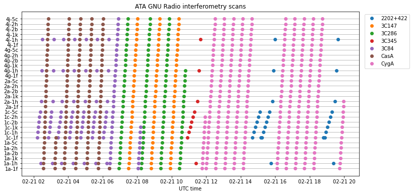
The 18 hour slot in which we had all the 12 antennas available was between 02:00 and 20:00 UTC on 2021-02-21. In this slot, we could observe Cassiopeia A from the beginning of the slot until the time it set, at around 06:00 UTC, and then observe Cygnus A from the time it rose around 11:00 UTC until the end of the slot (the ATA can track sources above 16.8 degrees elevation).
To do something useful between 06:00 and 11:00 UTC, when neither Cassiopeia A nor Cygnus A where up, Paul and I decided to observe some additional compact sources with all the possible baselines. This would serve as a way to verify phase calibration and the antenna coordinates. We used 3C147, which has a 6cm flux density of 7.9 Jy, and 3C286, which has a 6cm flux density of 7.5 Jy.
For the Cassiopeia A observation, scans of 30 seconds on the science target and 120 seconds on the calibrator were used. For the 3C147 and 3C286, we did 60 seconds scans. For Cygnus A we used 60 seconds for the science target and 300 seconds for the calibrators. In order not to spend too much time moving the antennas, we first moved all the antennas to the calibrator, iterated through the set of 10 baselines used for calibration, then moved all the antennas to the science target, iterated potentially several times through the set of 30 baselines, and then moved back to the calibrator. Between each calibrator revisit, the set of 30 baselines was iterated only once for Cassiopeia A and 5 times for Cygnus A.
The figure below shows the scans that were performed in the 18 hour observation. The pattern in which the scans were done is as described above, except for a few occasions in which we had problems with the software and had to restart it, which broke the observation pattern a little.
Software stack
FX correlator
The correlator is implemented as a software FX correlator in GNU Radio. Two dual-channel N32x USRPs are used to digitize the two polarizations of two antennas. The four IQ streams arrive into GNU Radio. Each of the streams is FFT-ed. Two things are done with the FFT outputs:
- The modulus squared of each FFT output is computed. This is used to compute power spectrums, which can be used for amplitude calibration.
- For each of the 6 possible combinations of pairs of FFT outputs, the product of one of the members of the pair and the complex conjugate of the other member is computed. Four of these 6 combinations yield the XX, XY, YX and YY interferometric correlations. The other two are single dish XY crossproducts, which can be used together with the XX and YY power spectrums to compute single dish Stokes parameters.
Each of these 4 real outputs and 6 complex outputs is integrated and decimated to an appropriate output rate. Finally, each of the outputs is saved in a GNU Radio metadata file which contains the timestamp, source name, observation frequency, and antennas used. Only the interferometric correlations will be treated in this post, and the imaging in CASA will be done with Stokes I on the XX and YY parallel-hands only. Doing a polarimetric calibration of this data and imaging the Stokes QUV parameters is something to try in the future.
The implementation of this correlator in GNU Radio is based on the correlator that I used in my polarimetric observations of 3C286. Only a few things were changed in the Python flowgraph that I used for that observation, so the interested reader can see that post for a detailed description of the correlator implementation. The Python flowgraph is in the polarimetric_interferometry.py script in the ata_interferometry Github repository that I’ve created to host this and future work.
The USRPs were run at 40.96 Msps. This was an improvement from previous interferometric observations, which were run at 30.72 Msps. By upgrading UHD from 3.15 to 4.0, we found a noticeable performance improvement. Whereas with UHD 3.15 we would get sample loss if running the correlator at 40.96 Msps, with UDH 4.0 we could run without problems. At 61.44 Msps we occasionally lost some samples. I tend to use even decimations of the 245.76 MHz clock, but by going to the 200 MHz clock we might be able to use 50 Msps. As I remarked in my post about 3C286, the bottleneck seems to be in the UHD Source GNU Radio block, since the system has many CPUs and the rest of the workload can be parallelized.
All the corrections for delays and phase rotation are done in post-processing, so the FFT size and the output rate must be high enough to prevent significant correlation losses. The maximum geometric delay with 300 metre baselines is on the order of 1us. The maximum non-geometric delay (cable delay) difference that we’ve measured is 1.65us, between antennas 1c and 5c. This means that the correlator must be able to cope with nearly 3us of delay. To do this without significant losses, we used an FFT size of 2048. At 40.96 Msps this gives an FFT length of 50us, so 3us of delay gives a correlation loss of only 6%.
Here it is important to remark that the correlation losses have two effects: first, they reduce the SNR, but more importantly, they reduce the visibility amplitude. Regarding SNR, we may or may not care too much. Even with 50% losses, a bright source is still bright. However, losing a 50% of the visibility amplitude would be a disaster for imaging. The good news is that in post-processing we know exactly how much delay we are correcting for, and hence how much correlation loss we have. Thus, we could scale up the visibility amplitudes to compensate for the losses.
However, it is better to have an FFT size that is large enough that no correction needs to be applied. The performance of the flowgraph hasn’t been impacted by increasing the FFT by a factor of 8 (in previous observations I used an FFT size of 256), since the FFTs are spread over 8 CPU cores. The only downside is the increase in the output data, but data reduction can be done just after correcting for the delay and phase rotation in post-processing.
Another simple way to solve this delay problem would be to set a constant delay correction for each scan, since the delay won’t change much over the course of a few minutes. However, I wasn’t able to get this working in time for the experiment, and we had the problem that we couldn’t determine the cable delays (which are as large as the geometric delays) in advance of the experiment.
The output rate of the correlator is set to 10 Hz. This is the same that I’ve used in the 3C286 observation and other interferometry experiments. The projection of a 300 metre east-west baseline at the equator would change at a maximum rate of 21 mm/s due to Earth’s rotation. This gives a phase rotation of 0.36 Hz at 4.9 GHz. The amplitude losses due to the output integration at a rate of 10 Hz are of only 0.2%. These amplitude lossess could be compensated in post-processing, in a manner that reminds of the sin(x)/x correction used with DACs.
Observation control
The observation control follows the same idea as in my observation of 3C286. A Python script instances the GNU Radio flowgraph, uses ata_control to control the array, and calls the flowgraph lock() and unlock() methods while changing the antennas in the IF switch matrix, moving the antennas, and closing and opening output files.
The script to observe Cygnus A and its calibrators is in observe_cygA.py. This was done well in advance of the observation and tested the weekend before with a reduced set of antennas. The script to observe the rest of the sources is in observe_casA_and_compacts.py. It was done a few days before the experiment, when we had finally settled on the exact slot where we could use the antennas, in order to make the best use of the slot as described in the observation set up above.
Something novel in these observation scripts is that all the calls to ata_control are wrapped in a function that will retry the call if it fails with an exception, instead of terminating the execution. Usually these exceptions are temporary errors, so we don’t want to abort an observation just because of them. Additionally, during tests we discovered that the rf_switch_thread() function sometimes got in an endless error loop, so we replaced it with set_rf_switch(), which is slower but doesn’t seem to give any problems.
Post-processing: phasing, data reduction and UVFITS
In post-processing, the output files generated by the FX correlator are first phased to the source. There is a separate set of files per scan, so post-processing is done on a scan-by-scan basis. The code used for phasing comes from my 3C286 and other interferometric observations, and can be seen in this Python function.
The antenna ECEF coordinates are used to form the ECEF baseline vector. The ICRS coordinates of the source are obtained with Astropy in the case of a catalogue source, or from a JSON file describing the observation sources in case the source is only given in terms of right-ascension and declination coordinates. The ICRS vector to the source gives the W vector. Orthogonal vectors due east and north in the image plane are computed to give the U and V vectors. For each timestamp in the FX correlator output (i.e., at a 10 Hz rate), all these three vectors are rotated to the ITRS frame with Astropy, and the projection of the baseline vector onto each of them is computed in order to obtain the UVW coordinates of the baseline.
The W coordinate is converted to cycles at the centre frequency in order to correct the phase rotation. It is also converted to seconds and added together with the fixed cable delay, which is used to correct for group delay by applying a linear phase slope over the FFT channels. No amplitude corrections for the correlation losses mentioned above are applied.
The phased visibility data is averaged to a resolution of 1 second and 640 kHz from the original resolution of 0.1 seconds and 20 kHz. This averaged data, together with the corresponding UVW coordinates and some metadata is written into a UVFITS file using pyuvdata.
These post-processing tasks are done in the grmeta_to_uvfits.py script, which performs the tasks described above to convert the GNU Radio metadata files generated by the FX correlator into UVFITS files that can be loaded into CASA. This script processes an input folder and iterates on a scan-by-scan basis, since the FX correlator generates separate output files for each scan. Additionally, the script performs other useful tasks such as rearranging the polarizations of baselines involving antennas 1c and 2b. During the observations it was discovered that the X and Y polarizations of these two antennas are swapped somewhere in the signal chain, so by rearranging the polarizations we correct this.
The grmeta_to_uvfits.py uses fringe_stop.py to perform the phasing to the source. This second script is something that I wrote earlier and forms part of an interferometric pipeline to process the voltage mode data of the CASPER SNAP boards at ATA into UVFITS for CASA. Together with Mike Piscopo and Wael Farah we are working on creating a pipeline to use the SNAPs instead of the USRPs for interferometry. The core of this pipeline is Mike’s X-Engine block. This implements the “X part” of an FX correlator (the “F part” being implemented by the PFB in the SNAP FPGA), and takes some ideas from xGPU, including the output format. Since most of the post-processing part is common between the USRP and SNAP pipelines, grmeta_to_uvfits.py reuses some code from the SNAP pipeline, and eventually it would make sense to turn both into a single tool.
CASA: calibration and imaging
The UVFITS files are imported into CASA, which is used for calibration and imaging. The procedure roughly follows the VLA continuum imaging CASA tutorial, with some variations due to the unique characteristics of the baseline-by-baseline sequence we do with the USRPs. The Python script that does all the processing in CASA is CasACygA_20210221.py.
The UVFITS files, each containing a single scan, are converted to CASA MS format and then all the MS files are concatenated. There is a quirk with this concatenation, which is that each concatenated file gets a different observation ID. It would make more sense to have the same observation ID for all the files, since each file already gets a different scan number. However, I haven’t been able to find how to change it without editing the MS tables by hand with browsetable().
After obtaining the concatenated MS file, bad data is flagged manually in plotms(). Then the flux density scaling is set for 3C286 and 3C147 using the C-band models distributed with CASA.
Bandpass calibration is done using 3C84, since it is much stronger than the other unresolved sources. First, a preliminary phase calibration is done. Since we’ve found that gain phases are usually stable for several hours, a single time-independent phase calibration is done for 3C84.
Due to the peculiarities of our observations with the two USRPs, delay calibration is not possible using CASA, since the delay calibration algorithm takes a single reference antenna and only uses baselines involving that antenna to measure the delays. Thus we are not able to measure delays for antennas on the same USRP as the reference antenna. Choosing a reference antenna on each USRP, we could make calibration tables for each of the USRPs, but then there is not an automated way to combine both tables. Since delays are small, however, they can be absorbed by the bandpass phase.
The bandpass calibration is done with a resolution of 4 channels (2.56 MHz), since otherwise there is not enough SNR to obtain good solutions for all the antennas.
After solving for the bandpass, a new time-independent phase calibration is done for 3C84. This is done to calibrate the X-Y phase offsets of each antenna, since the remaining phase calibrations are done in a polarization-independent manner (T gaintype). Since both polarizations are locked to a common clock, the X-Y phase offset is very stable, so doing a polarization-independent phase calibration is a good idea. On the other hand, the gain calibration is done in a polarization-dependent way, since the gains of the amplifiers in the signal chain are not tightly coupled.
To solve for time-varying polarization-independent phase, we use each of the unresolved calibrators (3C84, 3C286, 3C147, 3C345 and J2202+422). This needs to be done in a somewhat special manner to account for our baseline-by-baseline scans. In each solution interval enough baselines need to appear so that the gains of all the antennas can be solved. At first, I tried to use a fixed solution interval, such as 1 hour to guarantee that there is a full run of the calibrator inside each solution interval. However, this doesn’t happen, since the 1 hour segments are divided without regards to our observing cadence, so some segments would end up with not enough baselines. Thus, I have manually set time intervals for each solution, taking into account our calibrator runs. Usually, I have included two or three calibrator runs inside each solution interval in order to have good SNR in the calibration solution.
Once the phase has been calibrated in this way, a time-varying polarization-dependent amplitude calibration is done. Here the same manual solution intervals as in the phase calibration are used. Finally, the amplitudes are scaled according to the flux density scale for 3C286. All the calibrations are then applied to the data, and weights are computed from the variance by using statwt().
Imaging is done with a multi-scale CLEAN. A pixel size of 6 arcseconds, with a 256×256 pixels field for Cassiopeia A and 128×128 pixels field for Cygnus A is used. Cleaning masks, thresholds and iterations are determined by experimenting with interactive clean.
Results
To flag bad data manually, we have used plotms(). Some obvious problems such as very large or very small amplitudes can be seen by plotting amplitude versus time for all the fields and baselines. The calibrators are examined independently by plotting phase versus time for each baseline and flagging any outliers. With manual flagging, we have detected the following problems:
- A few minutes of Cygnus A correlations have very small amplitudes. The reason is unknown.
- All the baselines involving 1k have bad data for 3C147. The reason is unknown, and this is somewhat surprising, since the data for 3C286 is fine and these two sources have almost the same flux density.
- Other occasional outliers
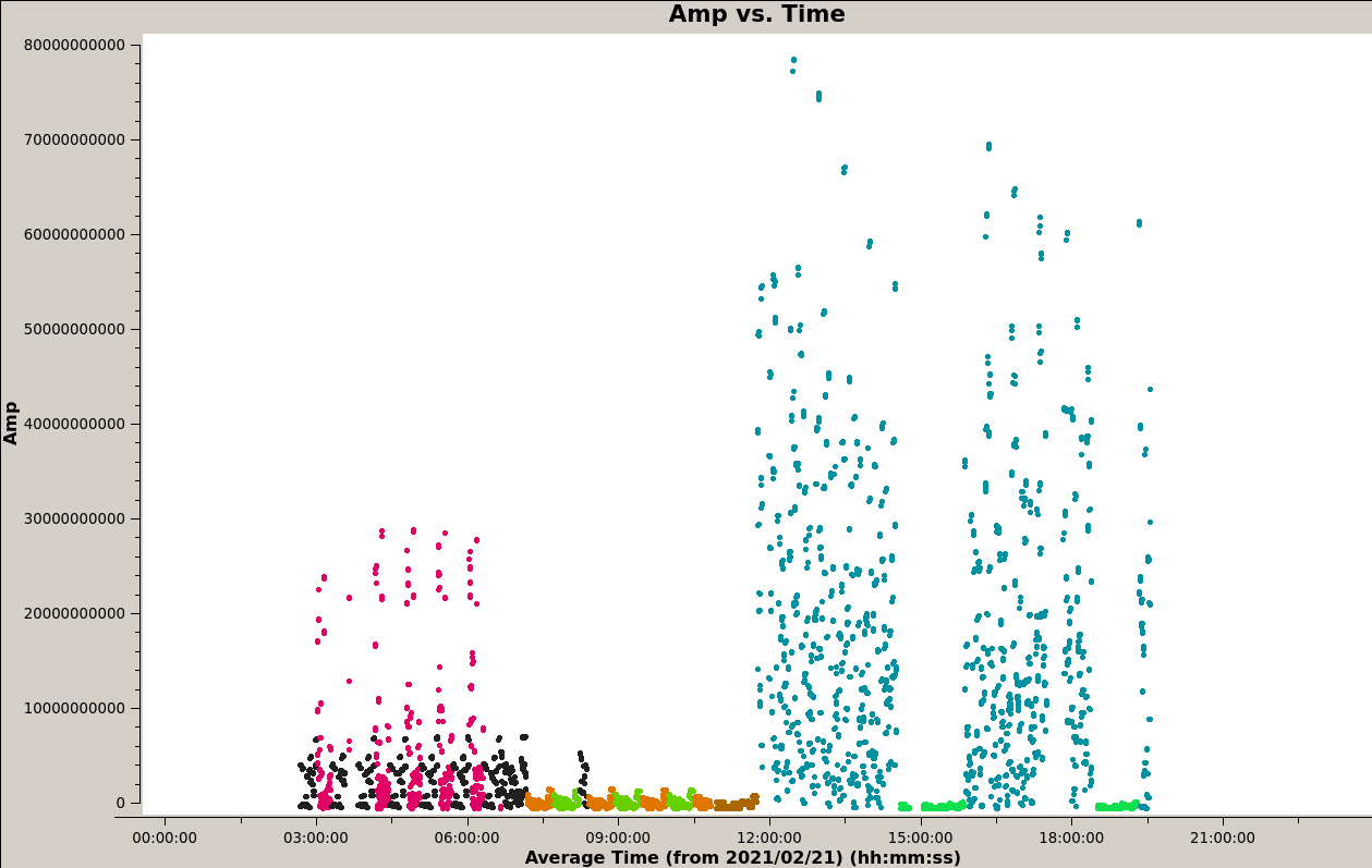
The uncalibrated amplitude versus time is shown in the figure below. The colour coding for the fields is as follows: 3C84, black; Cassiopeia A, magenta; 3C286, light brown; 3C147, green; 3C345, brown; Cygnus A, cyan; J2202+422, blue-green. Here we can already see the relative flux density difference between each of the sources.
The UV coverage for the science targets is shown below. Cassiopeia A is depicted in magenta, and Cygnus A is shown in cyan. We see that the UV data are clustered around a particular band for each of the sources. This is because the antennas of ATA are clustered along a NE-SW band, so longer baselines have roughly the same orientation. The bands for the UV coverage of both sources are different because they were observed at different hour angles. This shape of the UV coverage causes a large anisotropy of the synthesized beam.
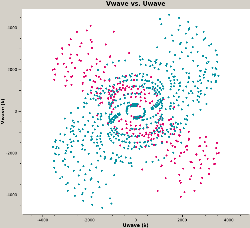
It is also convenient to note that the shortest baselines are on the order of 200λ. This makes features larger than 17 arcminutes be unresolved. The primary beam is several times larger than this, but our science targets are much smaller than this: Cassiopeia A’s size is 5 arcminutes, and Cygnus A is smaller.
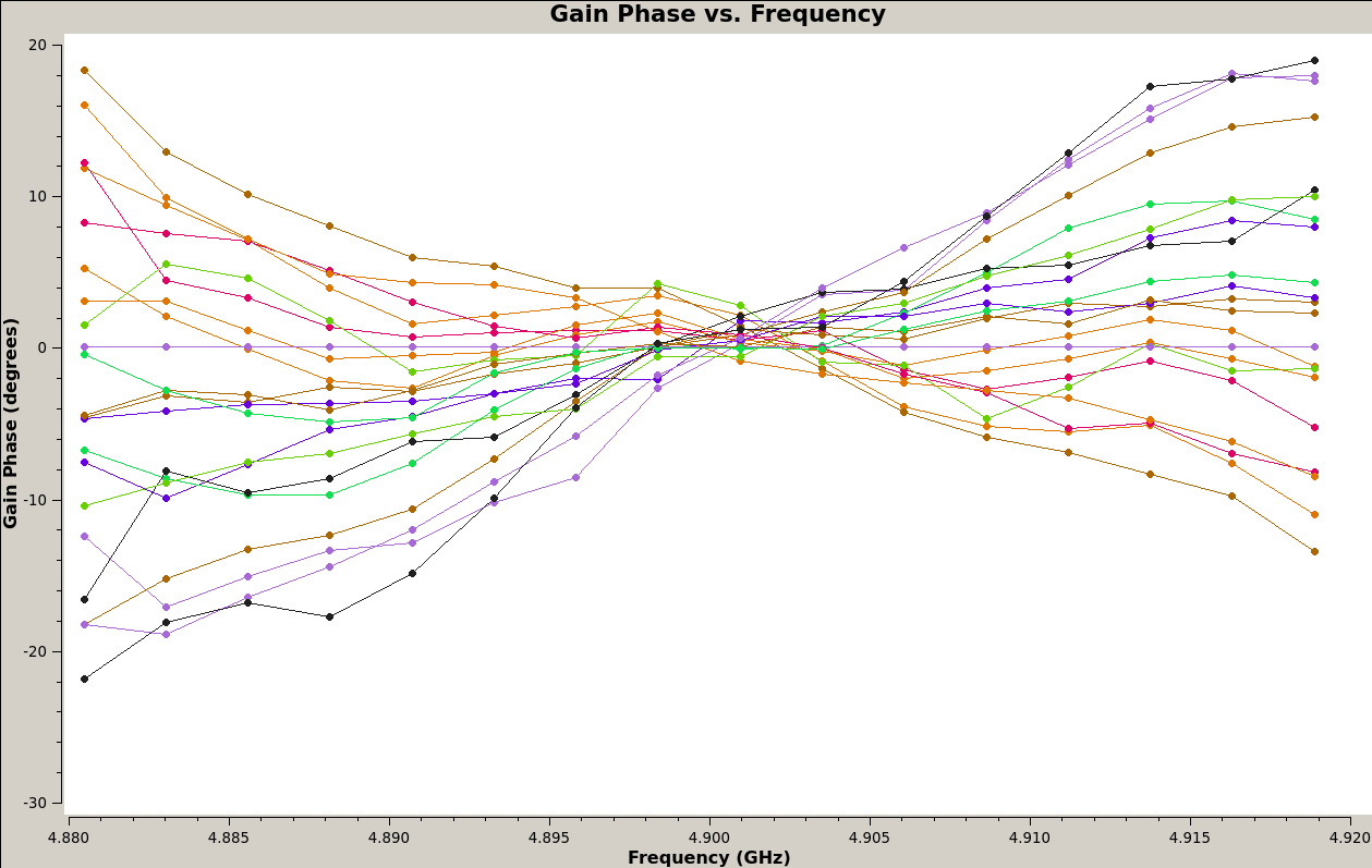
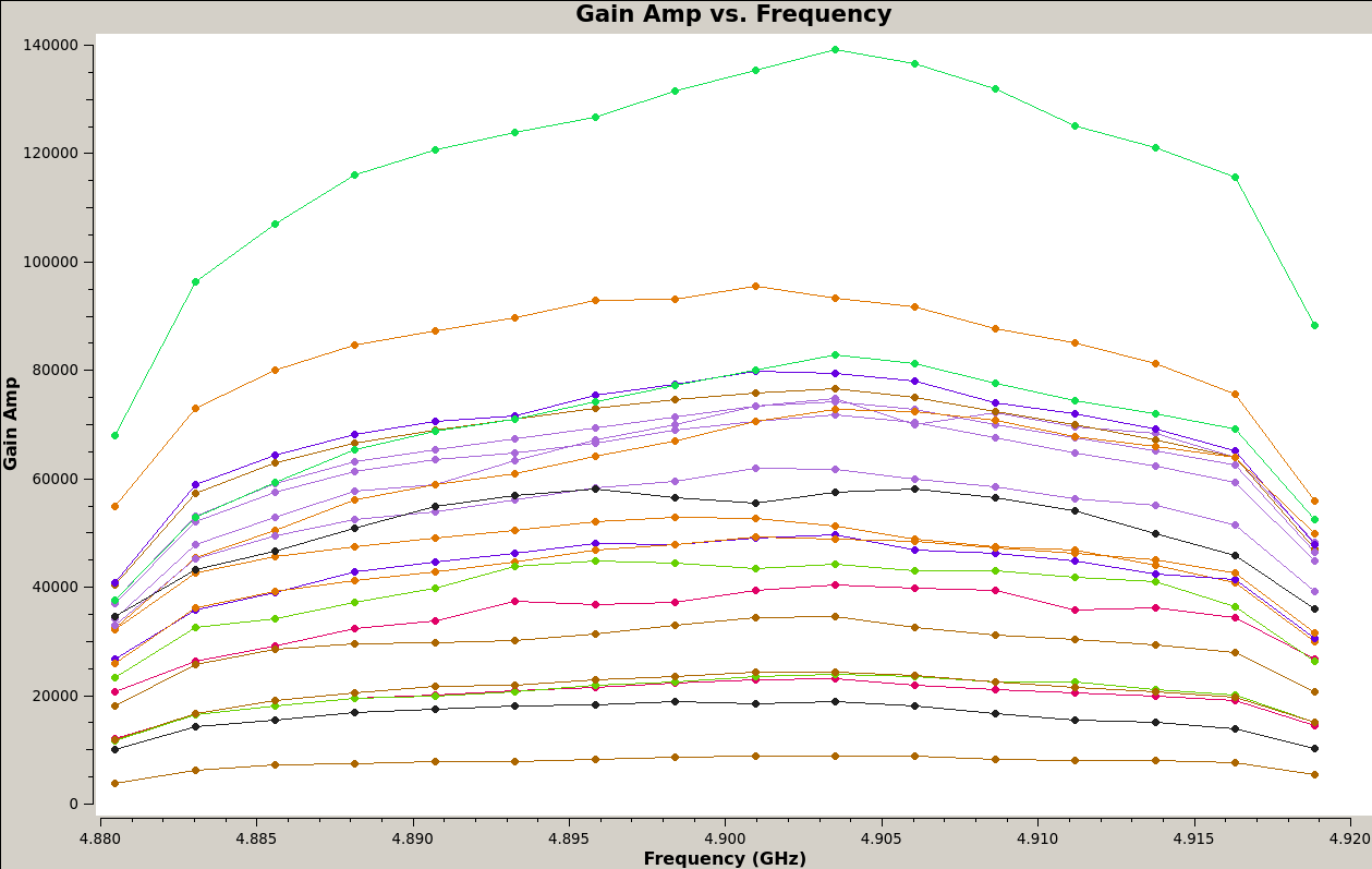
The next two figures show the bandpass calibration, with colouring per antenna. There are two traces with each colour, corresponding to the X and Y polarizations. As we mentioned above, we are not doing a delay calibration, so residual delays are absorbed by the bandpass phase. This gives a phase versus frequency slope. The maximum slope is of around 40 degrees over the whole 40.96 MHz bandpass, corresponding to a delay of 2.7 ns. The bandpass gain shows the typical shape of the USRP bandpass.
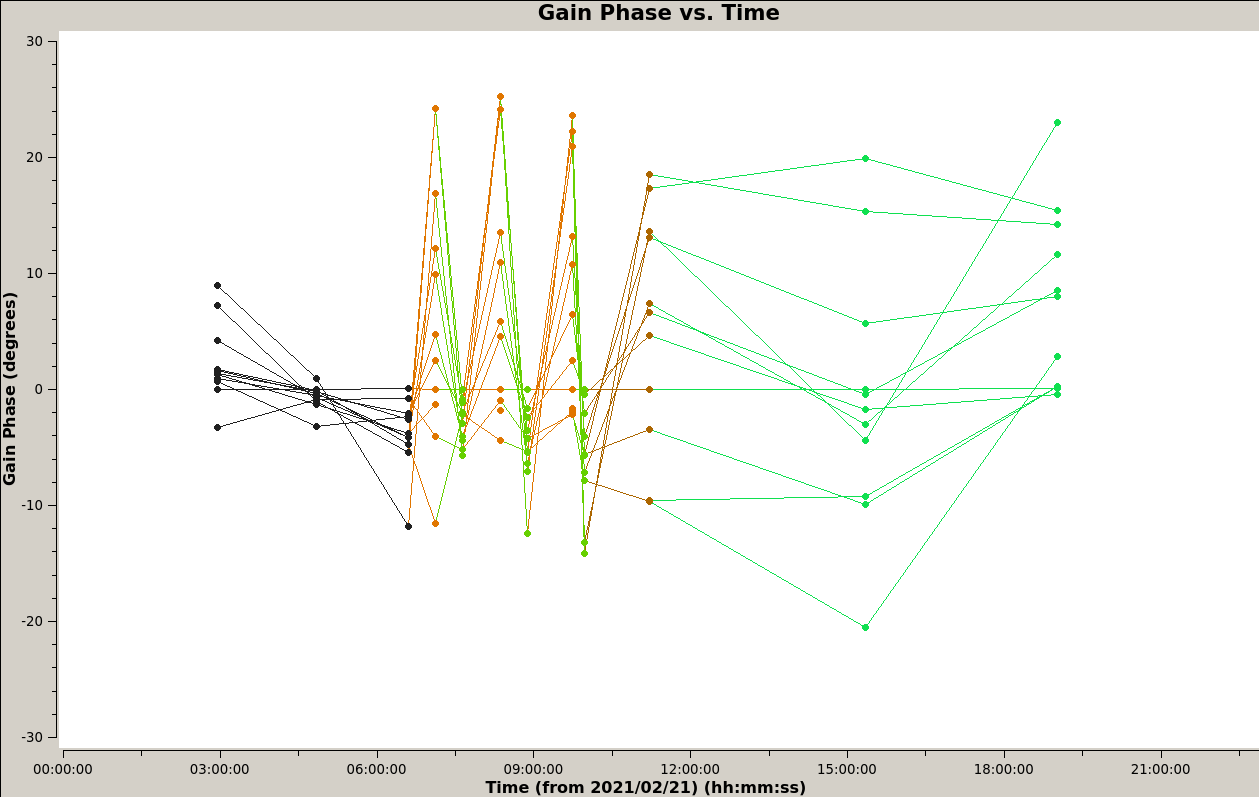
Below we show the polarization-independent phase calibration solutions. All the antennas are shown and colouring is by field. We see that there is a noticeable difference between the solutions for 3C84 and 3C147, and the solutions for the other unresolved sources. This points to direction dependent errors, which are probably caused by errors in the baseline coordinates.
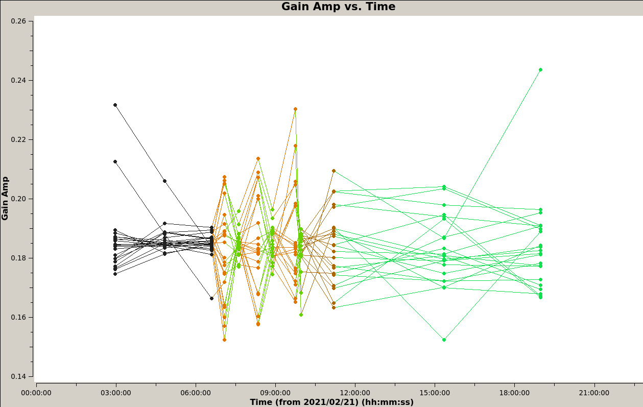
The gain calibration solutions show a certain variability, but there isn’t a clear correlation with time or with the observed source.
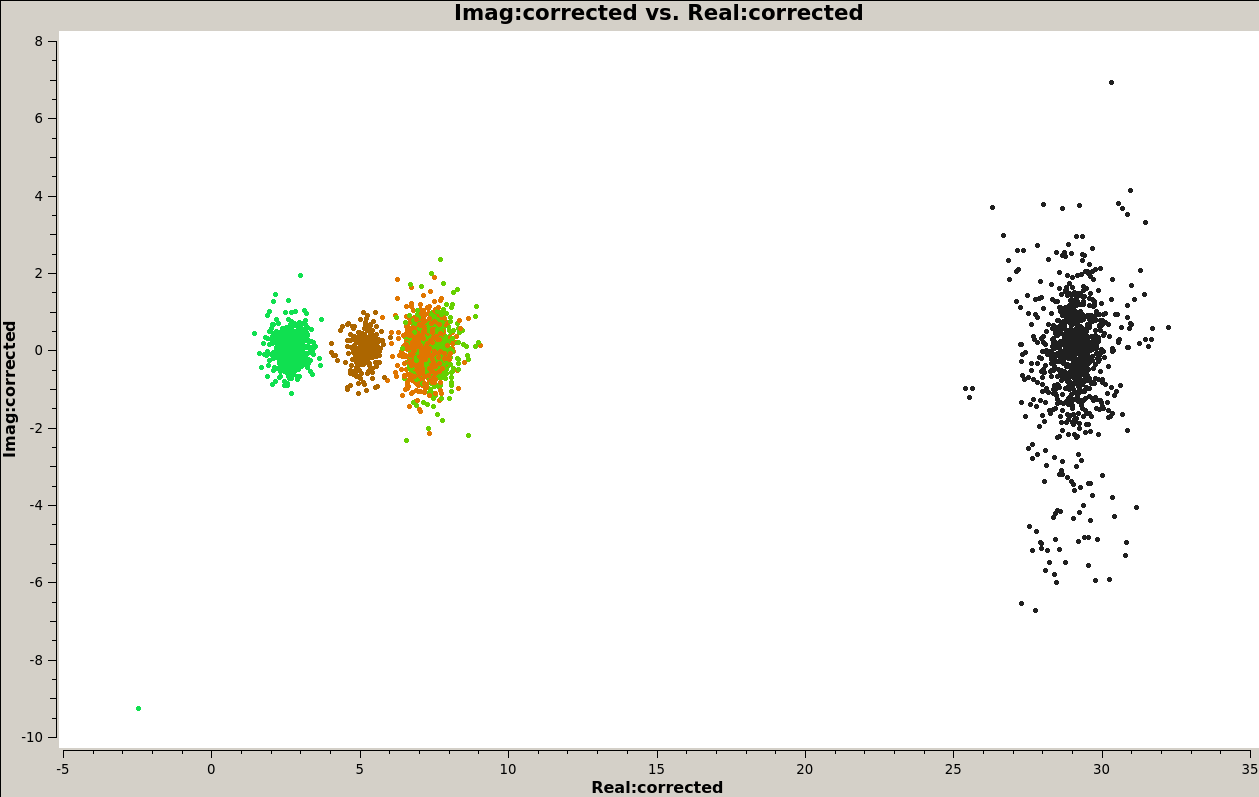
Calibrated visibilities for each of the unresolved sources are shown in the next figure. We see that the calibration has worked quite well and the visibilities for each source look like a normal distribution with mean equal to the source flux density. There are a few points for 3C84 (black) that appear to be outliers of this normal distribution, but none of them is too extreme.
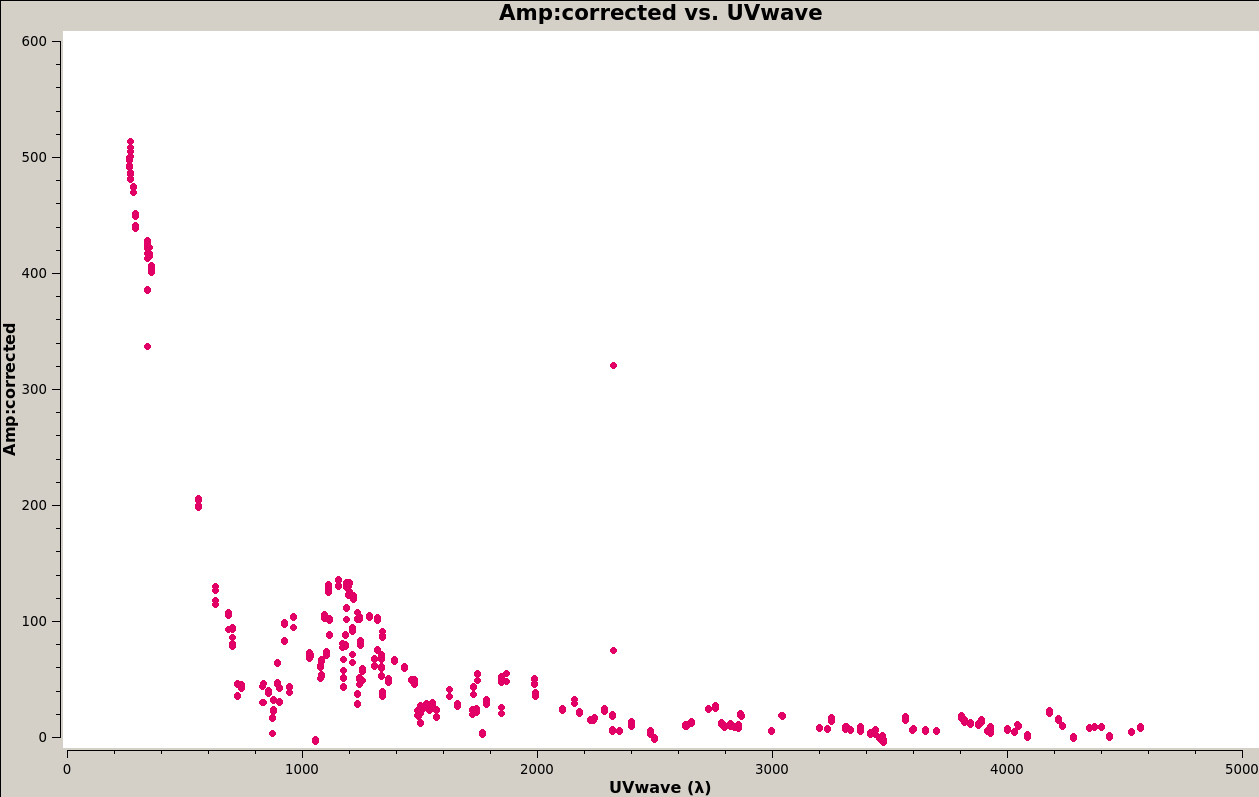
Below we show the calibrated visibility amplitude versus the modulus of (U,V). The visibility quickly drops down to a null at around 800λ, indicating a resolved component of around 4.3 arcminutes. This corresponds to the general extension of the supernova remnant. The part of the visibility plot below 800λ shows a strong dependency on the modulus of (U,V) only (and not on the angle of (U,V)). This is a consequence of radial symmetry. Then there are additional smaller maxima for higher modulus of (U,V), which give additional finer detail structure.
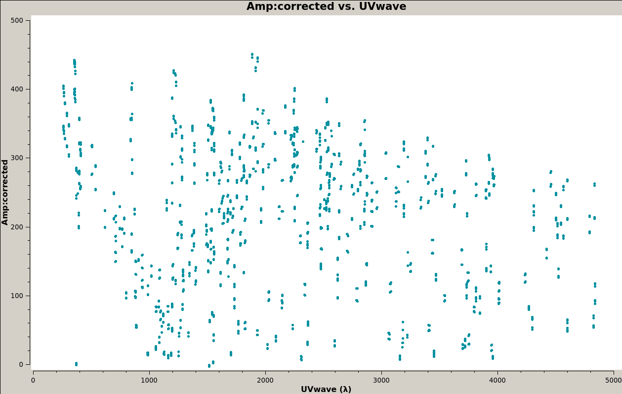
The visibility amplitude for Cygnus A is much harder to interpret. We know that Cygnus A is a double source, which breaks radial symmetry and makes the visibility depend on the angle of the (U,V) vector. We also see that the amplitude doesn’t drop down significantly at our largest 4900λ points in the UV plane that we are probing. This means that the main features are smaller than what we can resolve with ATA at this frequency.
The multi-scale CLEAN image for Cassiopeia A is shown below. The flux density is 504 Jy and the peak brightness is 33.8 Jy/beam. The synthesized beam is 109×31 arcseconds. The weaker components to the upper left and lower right are not real features of the source and are probably caused by sidelobes due to gain errors.
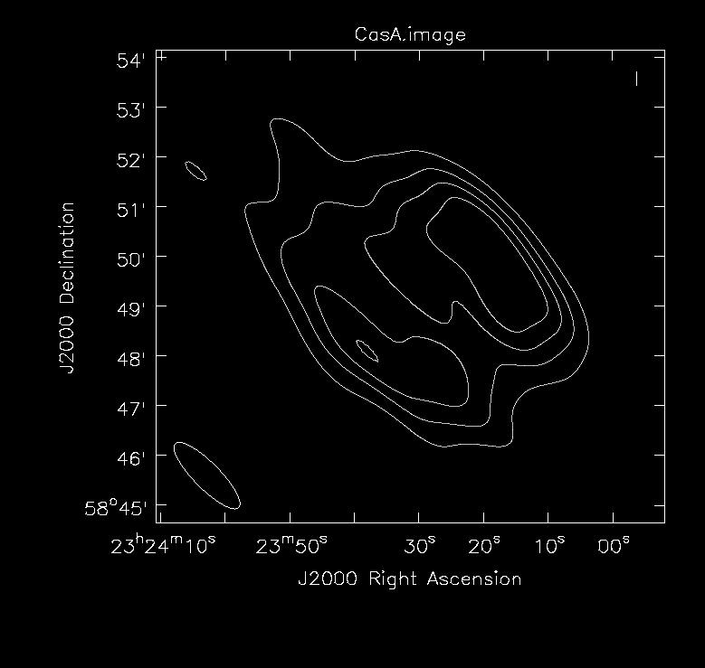
The corresponding contour plot is given below.
For reference, the figure below, taken from a paper by Perley and Butler, shows a higher resolution L-band image of Cassiopeia A. We see that our ATA image has accurately captured the higher brightness regions on the east and north parts of the supernova remnant, but the large anisotropic beam makes the image rather smeared.

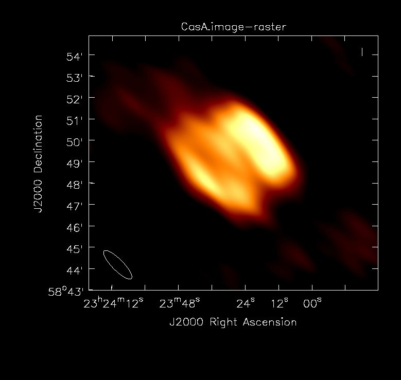
The next figure shows the multi-scale CLEAN image of Cygnus A. The flux density is 356 Jy and the peak brightness is 164 Jy/beam. The synthesized beam is 67×31 arcseconds. At this resolution, the source looks basically like two point sources, corresponding to the hot spots at the end of the jets.
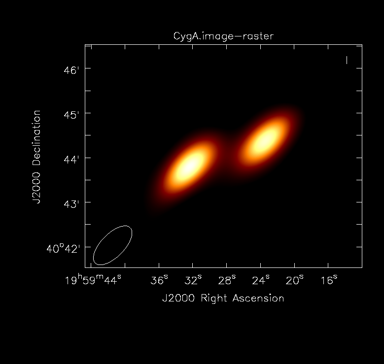
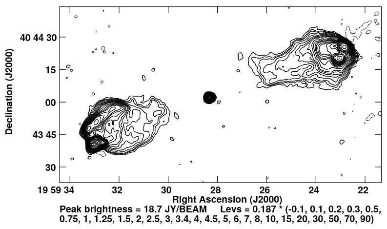
The contour plot hints that perhaps some of the flux in the central component, which corresponds to the radio galaxy itself, is captured in this image.

The Cygnus A image from the Perley and Butler paper is shown below for comparison. We see that at the resolution we have with ATA the hot spots at the end of the jets will look basically like point sources. The extended emission of the two lobes is much weaker and is not large enough to be resolved independently of the hot spots with a 30 arcsecond beam.
Data release
The data for this observation has been released in Zenodo as the dataset “Cassiopeia A and Cygnus A interferometric observation with Allen Telescope Array“. This includes the UVFITS files and the flags and CLEAN masks necessary to reproduce the CASA processing pipeline. The calibrated and reduced visibilities for Cassiopeia A and Cygnus A, as well as the images are also included. The raw FX correlator output size is 70 GB, so it is not included in the dataset.
Conclusions
This experiment shows the feasibility of using using a GNU Radio software FX correlator for interferometric imaging with a dozen of antennas from the Allen Telescope Array and two USRP N32x SDRs. The fact that with this setup only one baseline can be correlated at a time is a bit limiting and introduces some peculiarities in the observation scheduling and in the calibration. Nevertheless, it is possible to achieve good coverage of the UV plane by iterating over all the baselines over the course of 30 minutes or an hour.
The 300 metre longer baselines of ATA give a resolution on the order of 30 arcseconds at 4.9 GHz. This is good enough to image many interesting sources. Since all the long baselines are oriented along roughly the same NE-SW direction, it is important to use a large hour angle coverage. Otherwise the synthesized beam will be much larger than 30 arcseconds along its semi-major axis.
Here we show a complete description of the interferometric pipeline, covering from the IQ output of the SDRs to the CLEAN images. Therefore, this experiment is a valuable resource for anyone interested in learning about interferometry in radio astronomy.
One comment