Following my polarimetry experiments at Allen Telescope Array, on October 31 I did a polarimetric observation of the quasar 3C286 with two dishes from the array to use as a test-bed for polarimetric calibration. 3C286 is a bright, compact, polarized source, with a fractional polarization intensity of around 10% and a polarization angle of 33º over a wide range of frequencies, so it makes an ideal source for polarization calibration. It is the primary polarization calibrator for VLA. The observation duration was slightly more than 2 hours, and it was done around the transit of the source, so the parallactic angle coverage is large (around 90º).
My initial idea was to use this observation to perform a “single dish” polarization calibration of each of the dishes by separate (since the math is somewhat simpler) and then perform an interferometric polarization calibration. However, after initial examination of the data, the SNR doesn’t seem large enough to do a “single dish” calibration. The polarized signal from 3C286 is rather weak and is swamped by noise from other sources in the field and from the receiver, and also by gain variations in the receive chain.
On the contrary, the interferometric calibration has worked well, since correlating the signals from the antennas allows us to discard the uncorrelated receiver noise and to phase on the target and discard other signals from the field, by means of Earth rotation aperture synthesis.
In this post I give my analysis and results of the observation. I have done an ad hoc calibration in Python to determine the polarization leakage and measure the polarization degree and angle of the source, and also a full polarimetric calibration in CASA to compare my calibration with one obtained with professional software.
The data used in this post has been published in Zenodo as the dataset “Allen Telescope Array polarimetric observation of 3C286“.
Some references
While preparing this experiment, my main reference about polarization calibration has been ATA memo 87: “On-Axis Polarization Calibration with the ATA“. A paper by Sault and Cornwell about the Hamaker-Bregman-Sault Meausurement Equation has also been quite useful to understand the theoretical foundations. Wael Farah recommended me these lecture videos from Willem van Straten. I haven’t managed to watch all of them yet, but they seem quite interesting.
From a more practical perspective, the VLA polarimetry guide contains good advice about how to select appropriate polarization calibrators and perform enough observations to determine all the parameters.
Observation procedure
The raw data recorded from the observation consists of power spectral densities (self-spectra) and cross-spectra between the four channels (an X and a Y channel from each of the two dishes). Dishes 1h and 4g were used for this observation, with both of them using LO d in the RF converter board to downconvert to an IF of 512 MHz. A USRP N321 digitized the IF of dish 1h and a USRP N320 digitized the IF of dish 4g. The two USRPs were configured to use LO sharing between all the channels and were synchronized by means of the telescope 10 MHz and 1PPS signals. GNU Radio was used for all the digital signal processing.
The USRPs were set to a sample rate of 30.72 Msps, and a 256 point FFT was used to give a channel width of 120 kHz and to cover the expected geometric and instrumental delay between the two dishes without significant correlation losses. A coherent averaging interval of 0.1 seconds was used for the self and cross-spectra.
GNU Radio metadata files with detached headers were used to save the averaged spectra to disk, together with correct timestamps and other metadata. This has worked correctly in general, but for some reason some of the files do not have correct timestamps. Their first timestamp is zero, and then the timestamps continue increasing at one second per second (the metadata file sinks were configured to output one metadata header per second).
The observation was done at eight frequency bands: 1413 MHz, 1665 MHz, 2675 MHz, 4820 MHz, 6663 MHz, and 8665 MHz, taking advantage of the wide frequency range of ATA. To perform the observation, the LO was tuned to the first frequency and averaged spectra were collected in metadata files for 100 seconds. Then the data collection was stopped, the LO was tuned to the next frequency, and the data collection was restarted using new metadata files. This procedure was repeated iterating through the eight frequency bands several times.
This process was accomplished by runtime reconfiguration of the GNU Radio flowgraph. The flowgraph was paused, the LO was commanded to switch frequency, the existing file sinks were closed and deleted, and new file sinks were created and connected before resuming the flowgraph.
To run all the processing in real time in the gnuradio1 server at ATA, which has two Xeon Silver 4216 CPUs, the workload was split between several FFT blocks running in parallel. The cores of these processors are not particularly fast, but there are a total of 32 cores with 2 threads each. I made a rather general flowgraph directly in Python to experiment with different parameters trying to optimize performance. In the end, I settled on taking 100 ms blocks from each of the 4 input channels, having two FFTs per channel running in parallel, dispatching these 100 ms blocks to each of the two FFTs, running the multiplications and averaging also in parallel, and then combining the data again before saving to file.
The flowgraph is instanced and run from a Python script that controls the telescope with ATAcontrol and calls some methods of the flowgraph to perform the runtime reconfiguration of the file sinks whenever the frequency is changed. The Python script sets up the antenna LNAs, the RFCB LO and the IF switch, points the antennas on source, performs an autotune calibration of the PAMs and parks the antennas after the observation is interrupted. Thus, this Python script allows us to perform the observation in a completely automated way.
The observation was done for somewhat more than two hours around the transit of the source. This gives very good parallactic angle coverage, as shown in the figure below.

Observation pre-processing
The metadata files recorded during the observation are loaded up in this Jupyter notebook, which is used both for pre-processing and to perform the polarimetric calibration. The pre-processing consists of phasing the visibilities to the source to perform fringe-stopping. The phased visibilities are exported to UVFITS files for later processing with CASA.
For polarimetric calibration with Python, some FFT bins where RFI is present in the 1665 MHz band were masked out and removed in this step. The UVFITS files were not masked for RFI, since CASA has better automatic RFI flagging capabilities.
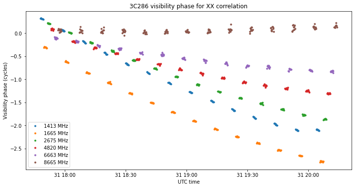
The baseline used for fringe-stopping comes from some L-band observations of Cassiopeia A and other sources done by Paul Boven and me in previous weekends. The baseline has been hand-optimized by some 20cm to improve the results for this observation. It is interesting that the optimal baseline solution seems to depend on the frequency, as shown by the figure below, which gives the unwrapped visibility phase after fringe-stopping. The fringe-stopping is very good for 8.6 GHz, but it is increasingly worse as we get lower in frequency.
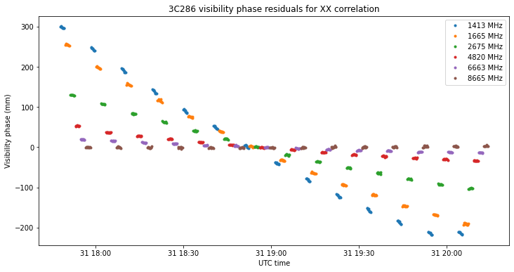
This is perhaps best seen by converting the phase to distance units and removing the average.
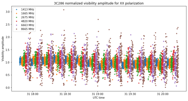
The normalized amplitudes show a clear decrease in SNR as we get higher in frequency. The reason is the spectral index of 3C286. Its flux density can be seen in the VLA flux calibration scale, and is around 15 Jy at 1.4 GHz, dropping down to 6 Jy at 6.6 GHz.
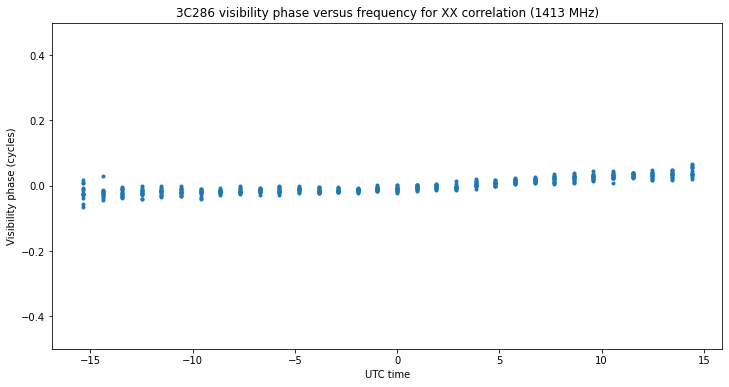
Plotting the phase versus frequency bin we can see that most of the geometric and instrumental delay between the antennas has been removed during fringe stopping. This allows us to average coherently all the frequency bins. The plot below corresponds to the 1413 MHz band. Other bands are similar, albeit with less SNR.
In this notebook, the fringe-stopped visibilities and their corresponding UVW coordinates and timestamps are saved to Numpy files for exporting to UVFITS files with pyuvdata (thanks to Andrew Siemion for suggesting this library). The export is done in this script. There is one quirk in this export: pyuvdata writes the antenna coordinates in a rotated ECEF frame so that the X axis goes through the local meridian. However, it seems that CASA doesn’t follow this convention and expects antenna coordinates in the usual ECEF frame when using importuvfits.
Therefore, I pre-rotate the antenna coordinates to cancel out the additional rotation done by pyuvdata. This causes pyuvdata to suspect that the UVW coordinates are wrong when checking the data and writing the UVFITS file, but everything works correctly despite the warnings given.
Polarimetric calibration in Python
The polarimetric calibration is described step by step in the Jupyter notebook, using many plots to show the intermediate results. Here I will focus on the mathematical background. The basic equation that we use is (2) from the ATA Memo 87:\[\begin{pmatrix}v_{xx}\\v_{xy}\\v_{yx}\\v_{yy}\end{pmatrix} \approx \frac{1}{2} \begin{pmatrix}g_{xx} & g_{xx} & 0 & 0\\g_{xy}(d_{1x}-\overline{d_{2y}}) & 0 & g_{xy} & ig_{xy}\\-g_{yx}(d_{1y}-\overline{d_{2x}})& 0 & g_{yx} & -ig_{yx}\\g_{yy} & -g_{yy} & 0 & 0\end{pmatrix} \begin{pmatrix} I\\Q\\U\\V\end{pmatrix}.\]
This equation relates to first order approximation the measured visibilities \(v_{xx}\), \(v_{xy}\), \(v_{yx}\), \(v_{yy}\) with the apparent source Stokes parameters \(I\), \(Q\), \(U\), \(V\) (appropriately rotated according to parallactic angle) and the complex gains \(g_{xx}\), \(g_{xy}\), \(g_{yx}\) and \(g_{yy}\), and D-terms (polarization leakage terms) \(d_{jx}\), \(d_{jy}\).
In our case, we can normalize the flux density so that \(I = 1\), and assume that the source has no circular polarization, giving \(V = 0\). Then \(Q = \rho \cos \alpha(t)\) and \(U = \rho \sin \alpha(t)\), where \(\rho\) is the polarization degree of the source and \(\alpha(t)\) is a function that depends on the source polarization angle and the (time-varying) parallacting angle.
The complex gains \(g_{xx}\) and \(g_{yy}\) are easily calibrated out by using the parallel-hand correlations \(v_{xx}\) and \(v_{yy}\). We can do a phase calibration that converts \(v_{xx}\) and \(v_{yy}\) into real and positive. Then, we can do a coarse amplitude calibration by using the power (self-correlation) measured in each of the channels to normalize \(v_{xx}\) and \(v_{yy}\) so that \(g_{xx}\) and \(g_{yy}\) are close to one. This gives that \(v_{xx} + v_{yy}\) is a good approximation of Stokes \(I\). Dividing out by this approximation to \(I\) we obtain a better gain calibration, so that now \(g_{xx}\) and \(g_{yy}\) are very close to one.
Looking now at the cross-hands, we see that for instance\[v_{xy} \approx \frac{1}{2}g_{xy} [(d_{1x}-\overline{d_{2y}}) + \rho \sin \alpha(t)],\]where we have used that \(I \approx 1\) and \(U \approx \rho \sin \alpha(t)\). Since the parallactic angle coverage is good, the function \(\sin \alpha(t)\) ranges over a relatively large interval of values between -1 and 1. This means that the cross-hand \(v_{xy}\) lies on a line in the complex plane described by \(a + g_{xy}\tau\), for \(\tau \in \mathbb{R}\). Here \(a = g_{xy}(d_{1-x} – \overline{d_{2x}})/2\).
Therefore, to perform a phase calibration of \(g_{xy}\) it is enough to find the angle of the line where the measurements \(v_{xy}\) lie. This can be done by fitting a line to the data. The amplitude calibration for \(g_{xy}\) can be done using the self-correlations, in the same manner as for the parallel-hand correlations. The same procedure can be applied to \(v_{yx}\), so after doing this calibration we can assume that \(g_{xy}\) and \(g_{yx}\) are close to one.
Now, the sum of cross-hands is\[v_{xy} + v_{yx} \approx \frac{1}{2}(d_{1x}-\overline{d_{2y}}-d_{1y} + \overline{d_{2x}}) + \rho \sin \alpha(t).\]The difference of the parallel hands equals, to first order approximation in \(g_{xx}-g_{yy}\) and \(\rho\),\[v_{xx}-v_{yy} \approx \frac{1}{2}(g_{xx}-g_{yy}) + \rho \cos \alpha(t).\]If we consider the points \(z = \operatorname{Re}(v_{xx} – v_{yy}) + i\operatorname{Re}(v_{xy}+v_{yx})\), we see that they line on a circle of radius \(\rho\). The centre of that circle can be used to estimate and calibrate out the residual difference of gain in the parallel-hands, \(g_{xx} – g_{yy}\), and the nuisance parameter given by the real part of the difference of D-terms, \(\operatorname{Re}(d_{1x}-\overline{d_{2y}}-d_{1y} + \overline{d_{2x}})\).
Once these terms are calibrated out, we note that the points \(z\) considered above are a good approximation for Stokes \(L = Q + iU\). From there, the polarization degree \(\rho\) and the apparent polarization angle of each measurement can be obtained. Performing the appropriate parallacting angle rotation, we can relate the apparent polarization angle on the sky to the true polarization angle of the source, and obtain an estimate for it.
The figure below shows the uncalibrated visibility amplitudes for one of the frequency bands. We see that there are large gain offsets and gain variations with time between the XX and YY correlations. These must be calibrated before trying to obtain any information from the difference \(v_{xx} – v_{yy}\).
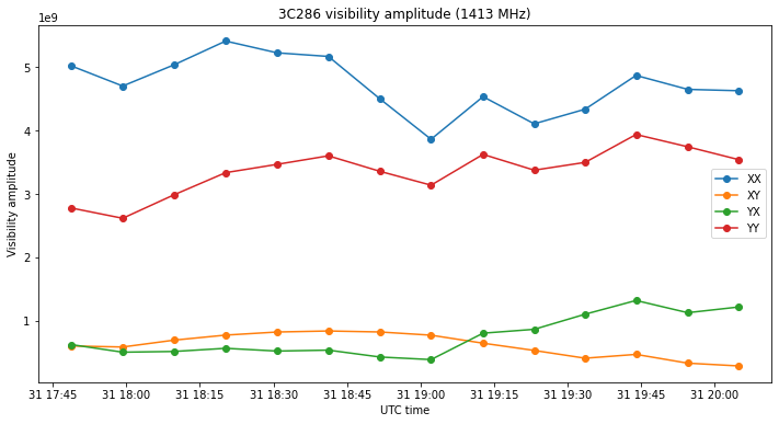
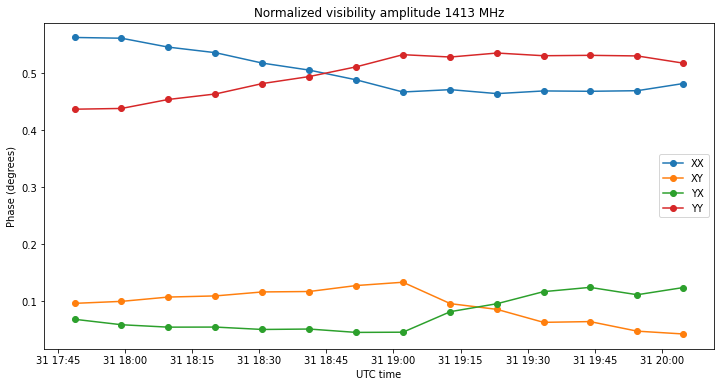
After calibrating the gains \(g_{xx}\) and \(g_{yy}\) we obtain the figure below, where we can now see how the XX and YY amplitudes cross each other as the apparent polarization angle of the source rotates on the sky. It is already possible to contrast this figure with the expected results given the known polarization angle of 33 degrees of 3C286 and the parallactic angle. However, the cross-hands \(v_{xy}\) and \(v_{yx}\) are still contaminated by leakage, so it is not possible to obtain any information from them yet.
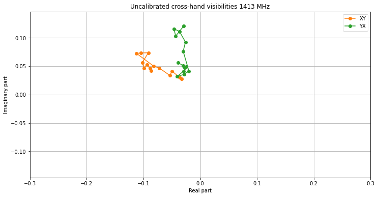
The figure below shows the uncalibratedd cross-hands \(v_{xy}\) and \(v_{yx}\) in the complex plane. We see that each of them lies on a line. The lines do not pass through the origin because of the leakage D-terms. From the angle of these lines we can obtain the phase calibration for \(g_{xy}\) and \(g_{yx}\). Here we also see that the D-terms are more or less of the same order of magnitude as the polarization degree of the source, so it is important to calibrate them out.
After calibrating the gains \(g_{xy}\) and \(g_{yx}\), we can plot the complex numbers \(z\) described above and fit a circle. The centre of this circle serves to refine the calibration of \(g_{xx} – g_{yy}\) and to remove the leakage D-terms.
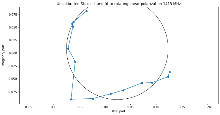
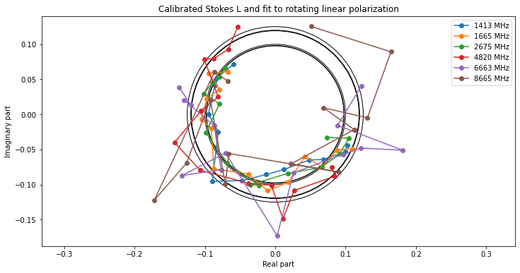
Finally, we obtain the calibrated Stokes \(L\) parameters, which lie on a circle centred in the origin. The radius of this circle is used as an estimate of \(\rho\).
Polarimetric calibration with CASA
This is the first time I use CASA, so I’ve mostly being following and adapting tutorials. The basic tutorial for non-polarimetric calibration that I’ve used is the VLA Continuum Tutorial for an observation of 3C391. This includes the calibration of the bandpass, delays, flux density scale, and complex gains. It also includes a section on imaging, which we won’t use here.
For polarization calibration I’ve followed the section about polarization calibration in the linear feed basis. It is convenient to remark that there are a number of tutorials on polarimetric calibration, but these use circularly polarized feeds, which have a rather different calibration procedure.
It turns out that the polarization calibration is essentially broken in CASA 6.1.0/5.7.0, as explained in the release notes. I wasn’t able to run CASA 5.6 on my system, so I’m using CASA 5.5.0 for the polarimetric calibration, and CASA 6.1.0 for the rest.
The non-polarimetric CASA 6.1.0 calibration script can be seen here. In this script we first import the UVFITS files as MS, set flux densities for 3C286 from the VLA models and apply automatic RFI flagging using tfcrop. This RFI flagging algorithm works pretty well for this data. The only major flagging is done in the channels of the 1665 MHz band that we had discarded above. Here we can see in the waterfall that the RFI is only sometimes present in the form of packet bursts (the waterfall doesn’t work in CASA 6.1.0 in my system, though, so I had to use CASA 5.7.0 to see it).
Then we do preliminary phase and gain calibrations in order to improve the data averaging for the bandpass and delay solutions. Some care needs to be taken with calibrations, because the SNR is not very high. In particular, I’ve needed to use the preavg parameter and to lower the minsnr parameter.
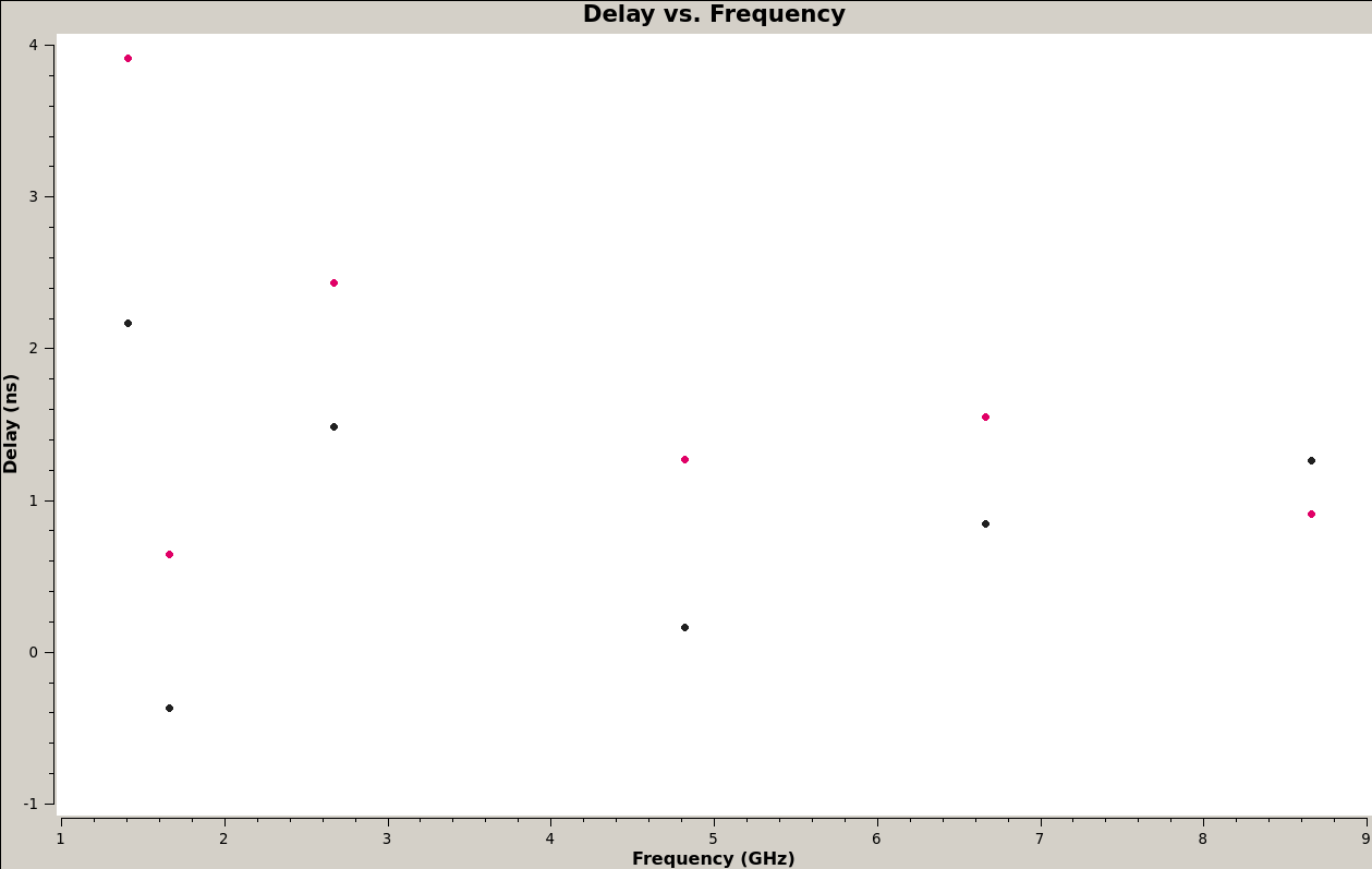
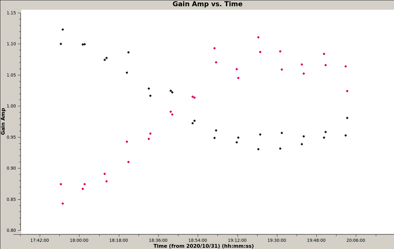
In all the calibrations, antenna 1h was used as the reference antenna. The figure below shows the delay solution for antenna 4g (with respect to the reference antenna 1h). We see that the fringe stopping is working well and the residual delay is only of a few nanoseconds. In all these plots, the black dots correspond to the XX correlations and the red dots correspond to the YY correlations. It is interesting to note that there is a noticeable difference of delays between the XX and YY correlations.
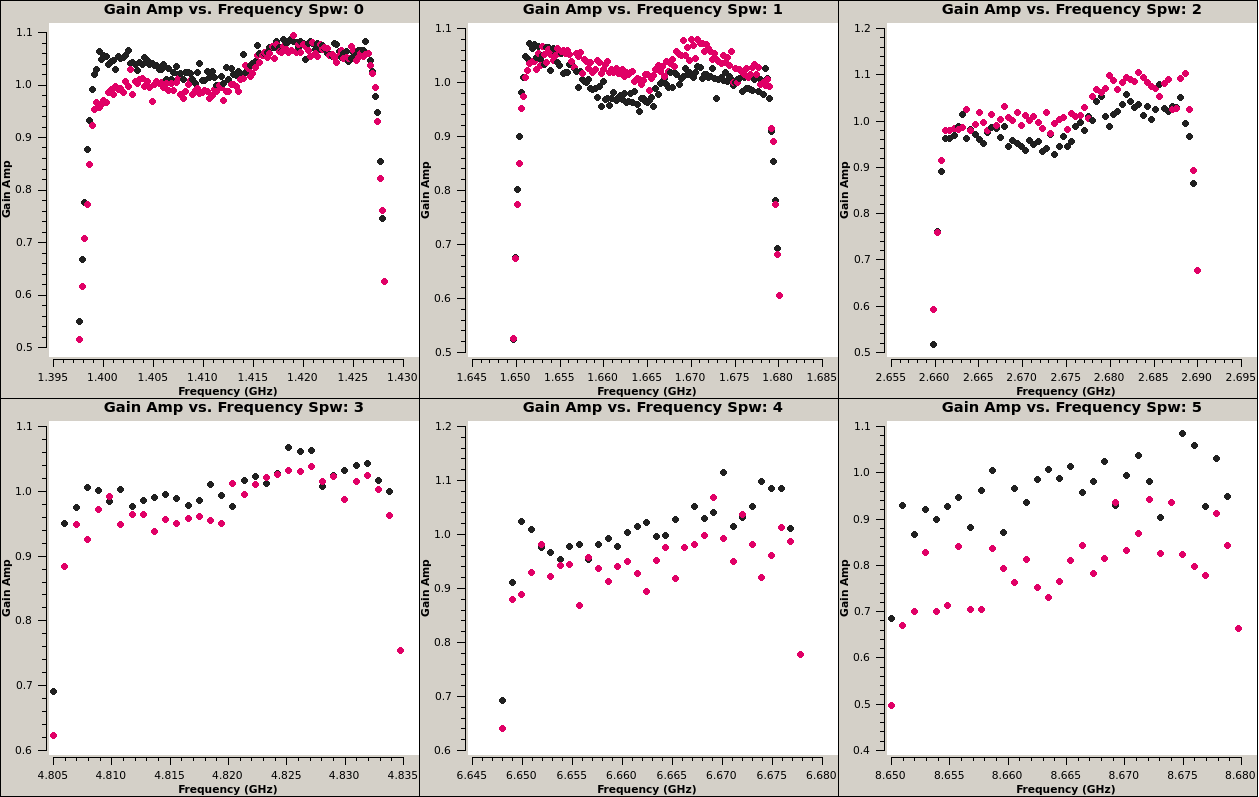
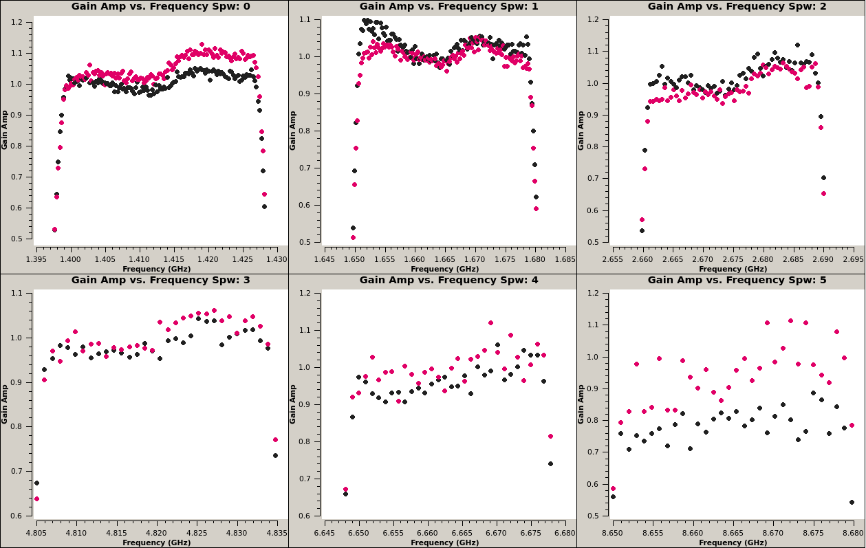
The figures below show the bandpass amplitude solutions for antennas 1h and 4g respectively. Since the SNR is lower in the higher frequency bands, I have used channel averaging for the calibration. Most of the shape of the bandpass seems to be caused by the USRP, particularly the asymmetry and the S curve shape in the middle of the passband. However, there are some other effects, since the bandpass calibration seems to depend on the frequency band, while the USRP is held always at the 512 MHz IF.
The figure below shows the bandpass phase solution for antenna 4g. This is really the phase difference between 4g and 1h, since 1h is used as a reference. The shapes obtained are quite similar to what I got in my GNSS interferometry experiment.
Once the delay and bandpass is solved, we do a final phase calibration. The results are shown below. This matches the phase drift rate that we had observed when examining the quality of the fringe stopping. However, we see that in the highest spectral window there is already substantial noise in the calibration.
Next we do a time-independent amplitude calibration with the goal of removing the amplitude difference between the X and Y channels. Care needs to be taken with amplitude calibration because the parallactic rotation of the source causes changes in the amplitude of X and Y that we don’t want to absorb in the calibration.

To absorb the polarization-independent amplitude variations, we do a polarization-independent (tropospheric) amplitude calibration. We see that especially the 1413 MHz band has some significant amplitude variations.
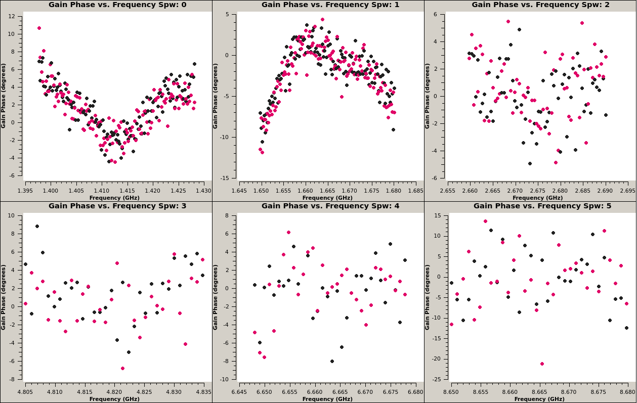
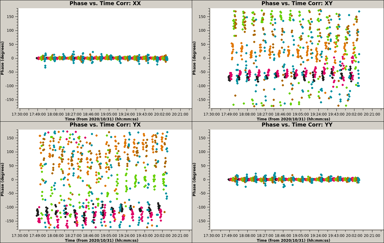
After non-polarimetric calibration, the data is averaged to 10 second intervals and every 8 frequency channels are averaged together, to give a frequency resolution of 960 kHz. The figure below shows the phase of the calibrated data. Colouring is by spectral window. The phase of the parallel-hands is almost zero, as expected. The phase of the cross-hands is not zero, mainly because the X-Y phase offset has not been calibrated yet.
Below we see the amplitude of the calibrated data. The colouring is by spectral window. Higher frequency spectral windows have less amplitude because 3C286 has less flux at higher frequencies. We can already see how the XX correlation slopes down over the course of the observation, while the YY correlation slopes up.

To perform polarimetric calibration, the data is normalized to unit flux, which simplifies the procedure. The first step involves doing an amplitude calibration of the parallel hands to extract a preliminary estimate for the source Stokes parameters. Such a gain calibration is shown here for the first spectral window.
Next, a calibration of the cross-hand delays is done. Only the three lower spectral windows are calibrated. For the three higher spectral windows, the SNR in the XY and YX correlations seems to be too low and the calibration gives nonsensical very high delays. The results shown below for the three first spectral windows make sense.
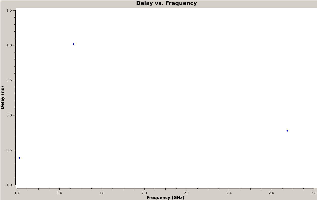
The cross-hand delay solution is not used for subsequent calibrations, since the absence of data in this table for some of the spectral windows causes problems.
The difference in gain calibration of the XX and YY parallel-hands is used to estimate the source Q and U Stokes parameters with the qufromgain script. Then the X-Y phase offset and the source Q and U Stokes parameters are solved from the cross-hand data. There is a 180º ambiguity in solving the X-Y phase offset. We had already encountered this ambiguity in our ad hoc calibration in Python. The ambiguity is resolved by comparing with the results of qufromgain. This yields a model of the source Stokes parameters.
Even though qufromgain is able to estimate reasonable Q and U parameters for all the spectral windows, the X-Y phase offset calibration and QU estimation using the cross-hands gives erroneous results for spectral windows 3 and 5. This makes the subsequent polarization calibration for these spectral windows give incorrect results, since we are using a wrong source model.
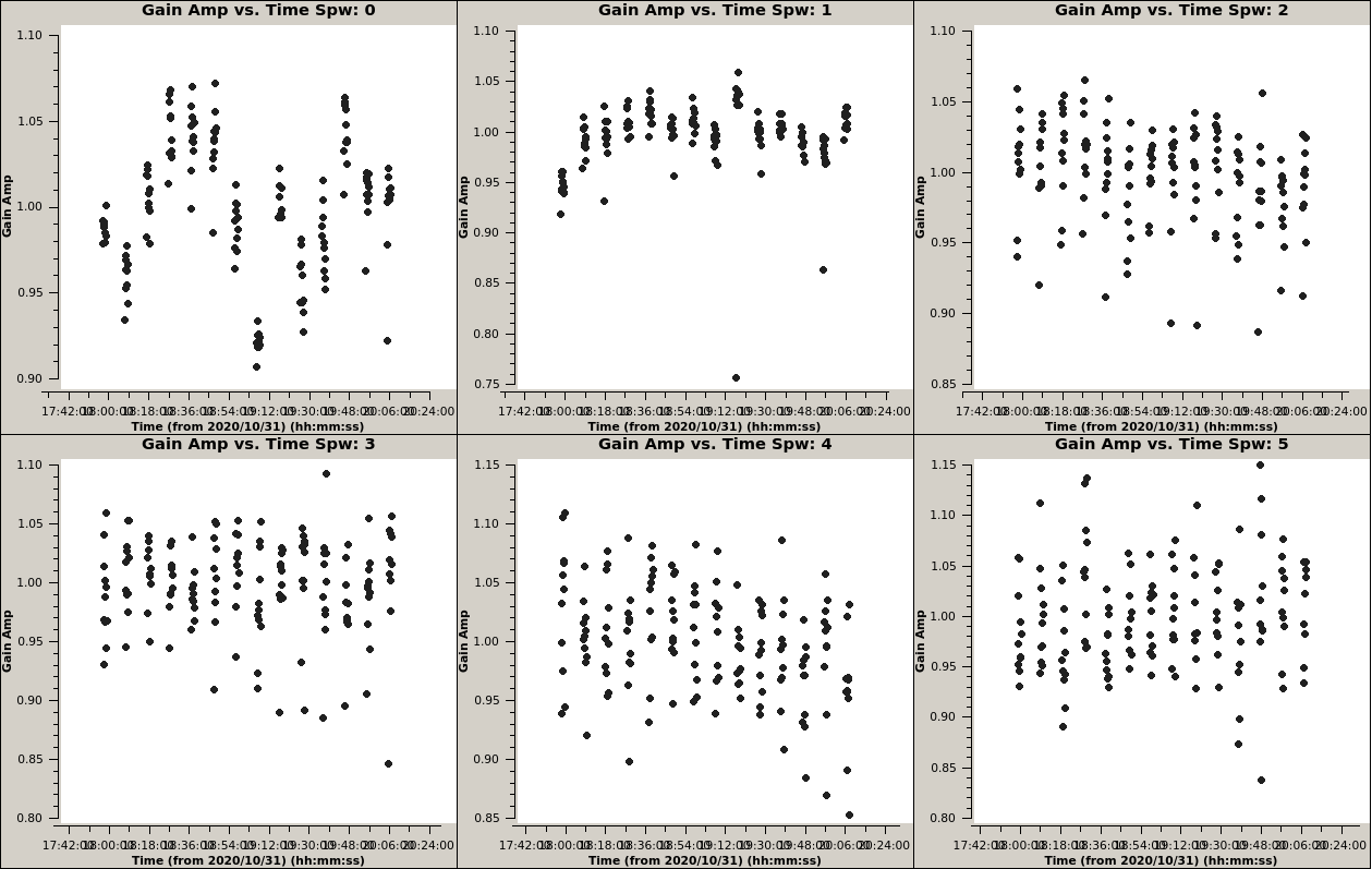
After the source Stokes parameters have been determined, an amplitude calibration taking into account the source polarization and the parallactic angle rotation is done. The source model seems good, since the gain solution is not absorbing the rotation of the apparent source polarization.
Next we do a D-term calibration, whose results are shown below. Note that spectral windows 3 and 5 are showing nonsensical results.

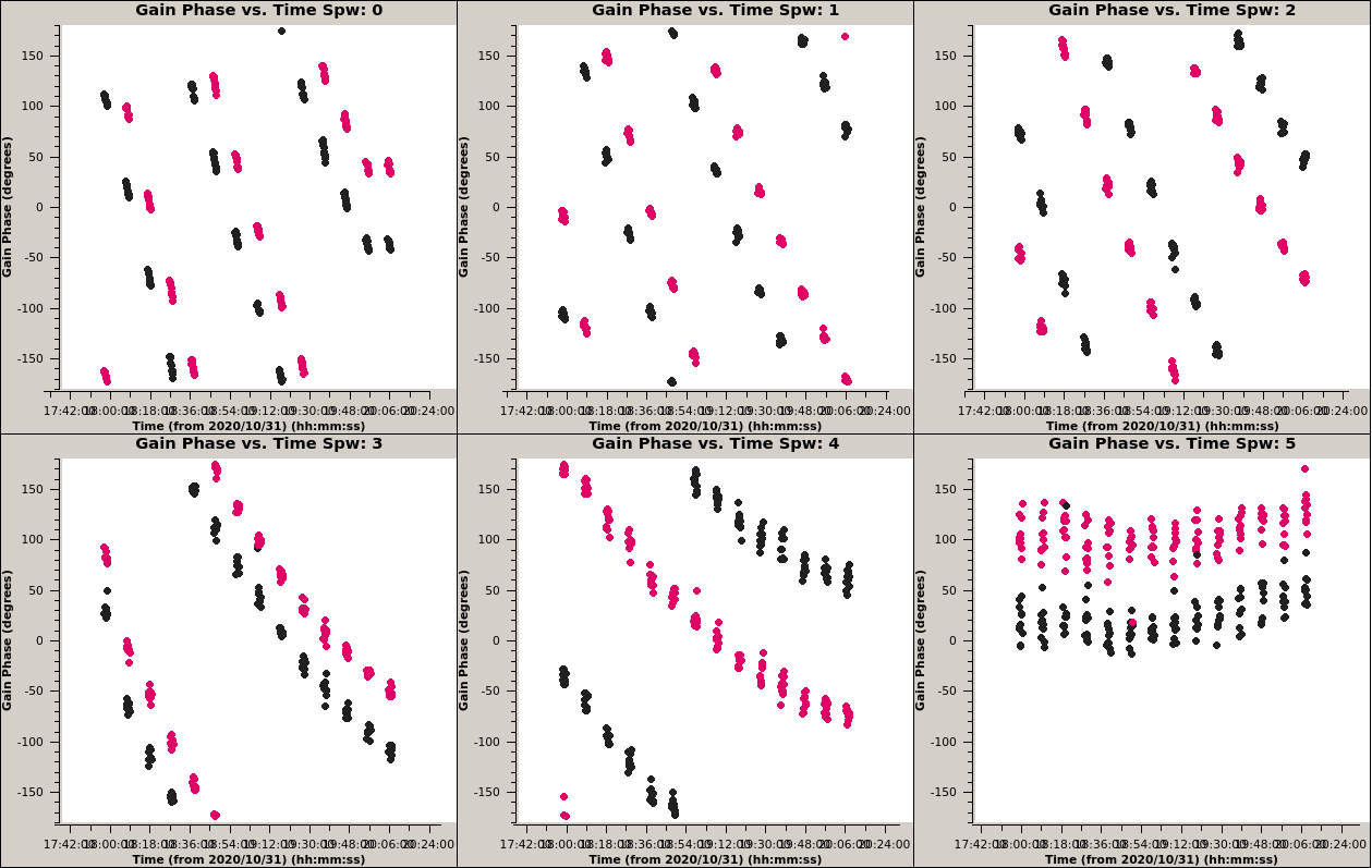
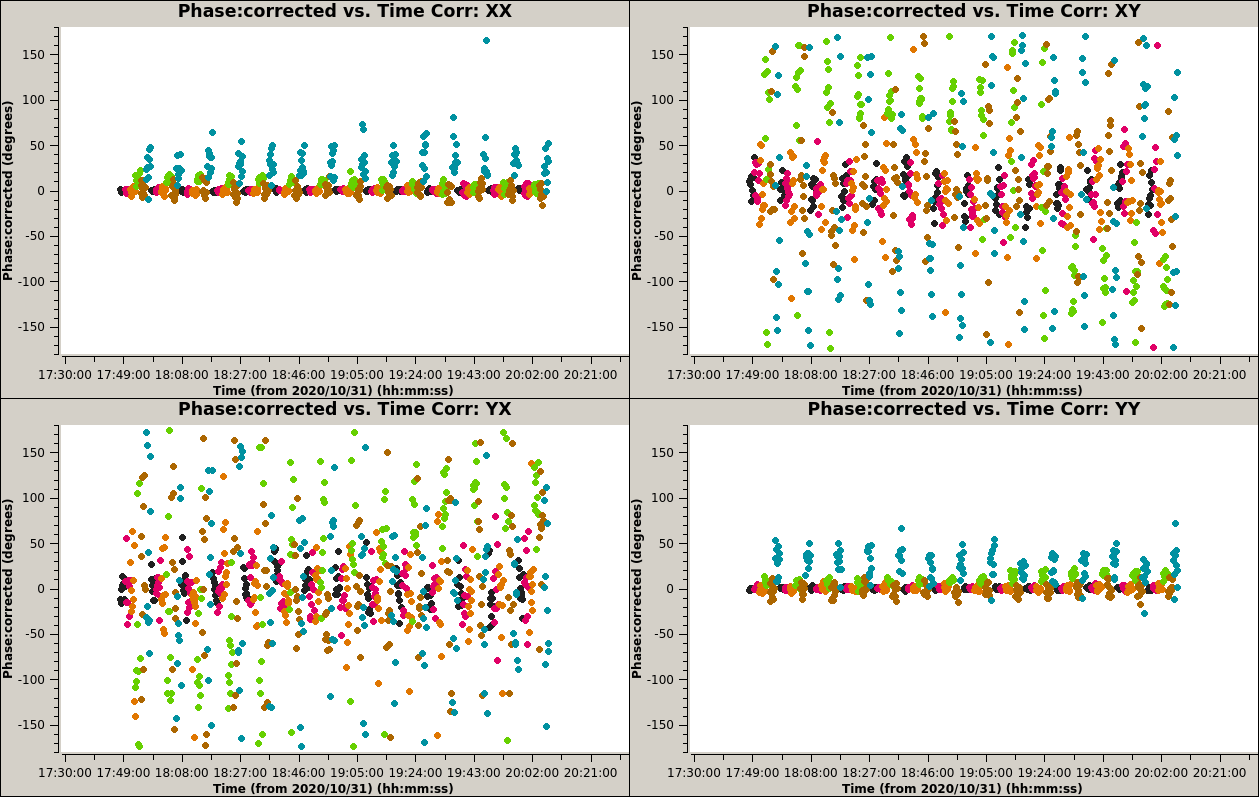
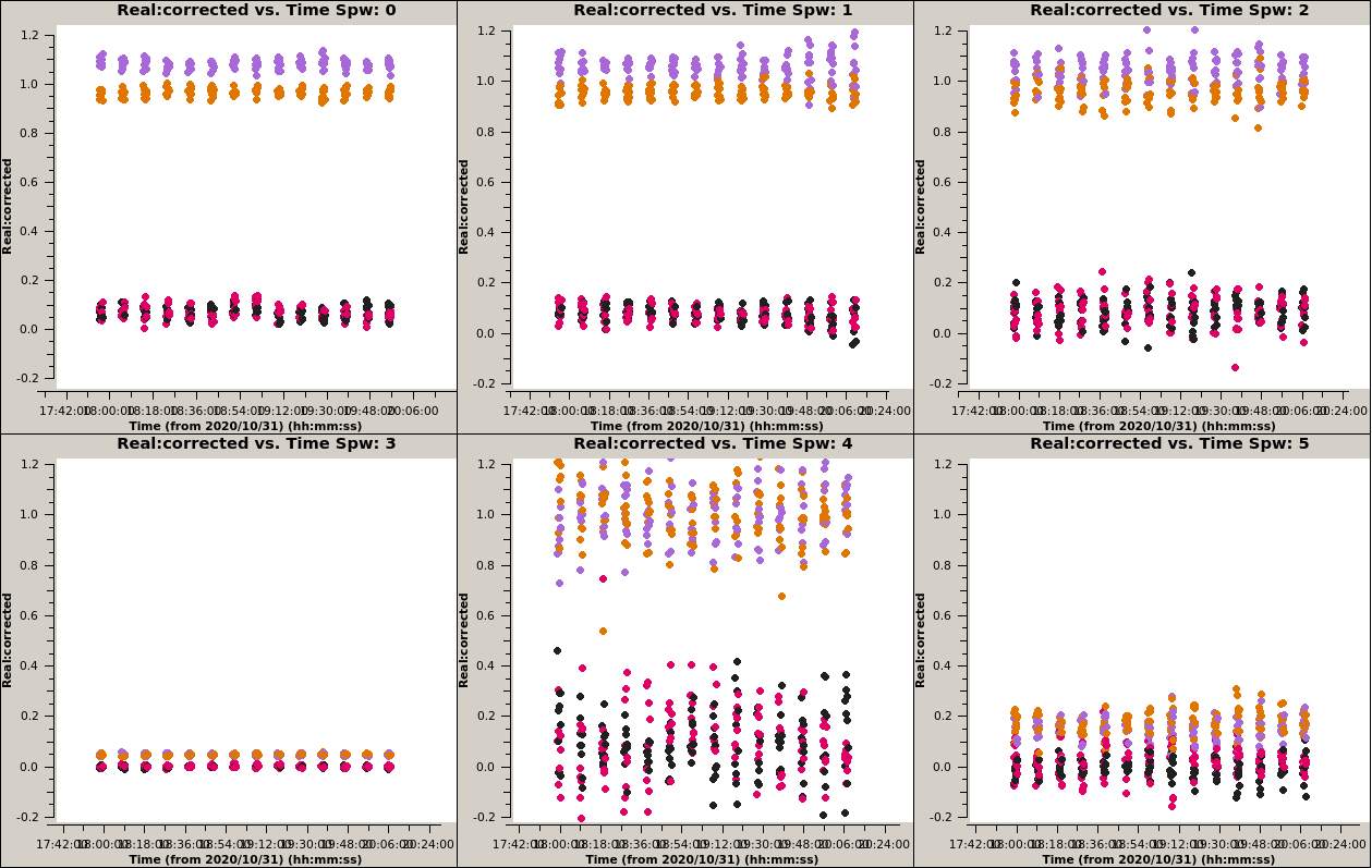
Finally, all the above calibrations are applied to the data accounting for parallactic angle rotation. This should yield correlations that follow the source Stokes parameters. The figure below shows the phase of the fully calibrated data. The phase of spectral windows 3 and 5 is somewhat wrong for the XX and YY correlations, and all over the place for XY and YX. This is caused by the incorrect polarimetric calibration.
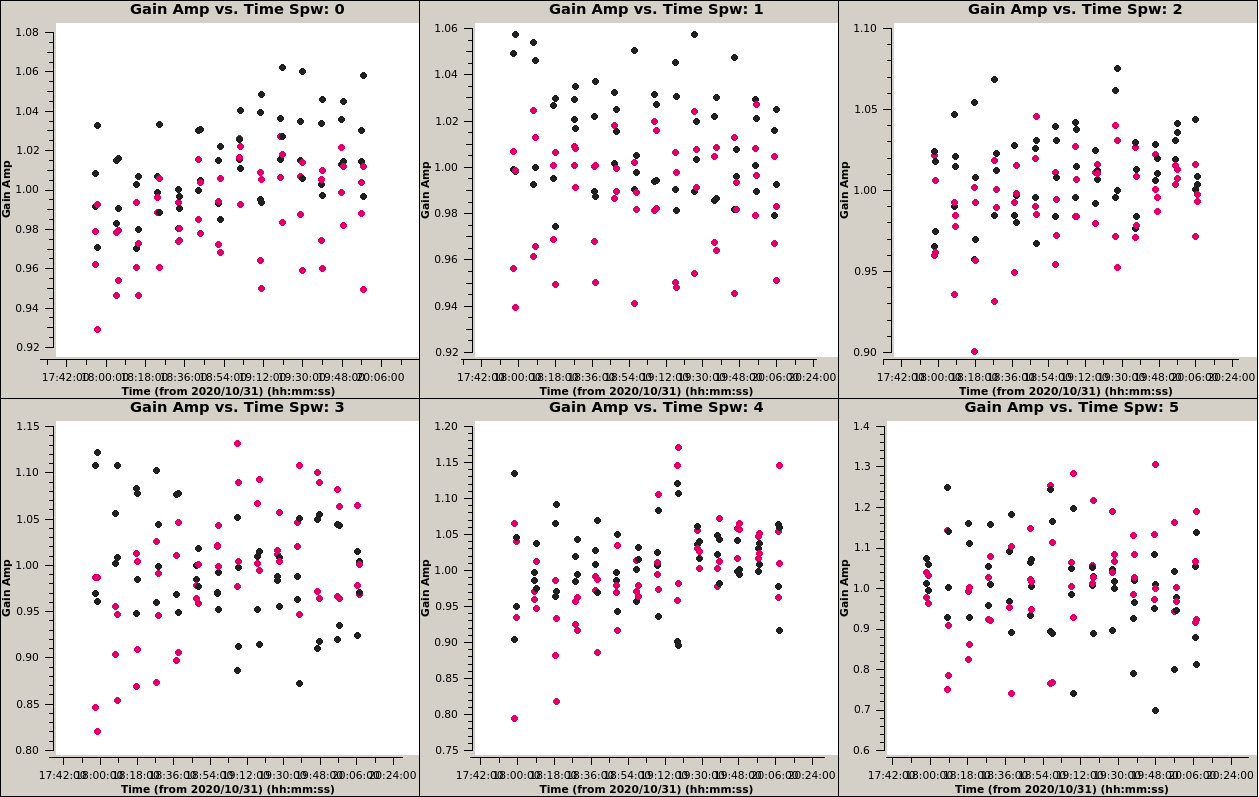
The next figure shows the real part of the visibilities, from which the Stokes parameters can be directly read off. Spectral windows 3 and 5 are clearly wrong because the phase is wrong, as shown above. Spectral windows 0 through 3 show good results that are constant with time, despite the source parallactic angle rotation. Even spectral window 4 looks good, albeit quite noisy.
The scripts used in this section are 3c286_casa.py for the non-polarimetric calibration in CASA 6.1.0, 3c286_casa_pol.py for the polarimetric calibration in CASA 5.5.0, and 3c286_casa_plots.py to produce the plots shown above.
Comparison of results
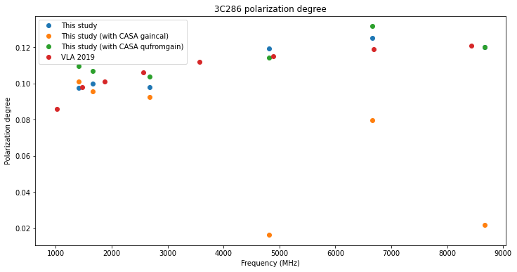
The end of the Jupyter notebook includes some plots that compare the ad hoc calibration in Python, the results obtained in CASA, and the measurements done at VLA in January 2019. For the results from CASA we show both the result obtained by gaincal, which performs a calibration of the X-Y polarization offset as well as an estimate of the Q and U Stokes parameters of the source, as well as the result obtained by qufromgain, which estimates Q and U from the difference of gain in the parallel-hands.
Regarding the polarization degree, we see that for the three lower frequency bands the results obtained by the Python notebook and CASA match quite well the data from VLA. For the three higher spectral windows the result obtained by gaincal is quite wrong, while the result obtained by qufromgain and by the Python notebook is in line with the VLA data.
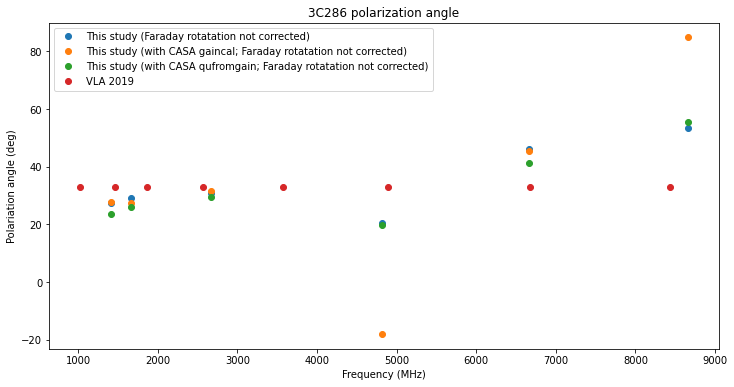
For the polarization angle it is important to remark that we haven’t estimated and corrected the ionospheric Faraday rotation. As shown in this paper, during solar minima the rotation on L-band is usually smaller than 5 degrees. It decays with the square of the frequency, so its effect is negligible for the higher frequency bands.
For the three lower frequency bands the results are quite near the VLA measurements. For the 4820 and 8665 MHz bands the result of gaincal is wrong, as we already noted. However, qufromgain gives very similar results to the Python notebook, even though they are quite different from the VLA measurements for some bands.
Concluding remarks
The results from the interferometric polarization calibration using 3C286 have been quite good, especially for the three lower frequency bands, which have better SNR. The Python notebook gives good geometric insight about what steps are involved in the calibration, while CASA allows us to do more advanced and automated processing.
The higher frequency bands gave some problems regarding low SNR because of the spectral index of the source. In hindsight, it would be a good idea to select a much brighter source for bandpass and delay calibration. The cross-hand delay is another aspect to be improved. It can be calibrated on any linearly polarized unresolved source. I wonder if there is another better candidate that gives higher polarized flux than 3C286. Finally, using longer scans for the higher bands would help.
The polarimetric calibration in CASA was problematic for the higher spectral windows. It should be possible to use an a priori model of the source Stokes parameters to help the calibration, and also to iterate the calibration solution once an improved source model is obtained.
The apparent frequency dependence of the baseline solution required to achieve fringe stopping is something strange that remains unexplained yet. We are currently investigating this, since we need to have good baselines for a set of different frequencies for a number of ongoing and future projects.
The single dish polarimetric calibration seems rather difficult to do with this kind of data. Whether there is a better approach remains open. I have considered using satellites instead of astronomical sources (an idea with which I already experimented in my GNSS polarimetric observations), but the difficulty seems to have a good a priori model for the source Stokes parameters (i.e., how perfect is a nominally circular polarization).
2 comments