This post belongs to a series about the activities of the GNU Radio community at Allen Telescope Array. For more information about these activities, see my first post.
The feeds in the ATA dishes are dual polarization linear feeds, giving two orthogonal linear polarizations that are called X and Y and (corresponding to the horizontal and vertical polarizations). In the setup we currently have, the two RF signals from a single dish are downconverted to an IF around 512 MHz using common LOs and then sampled by the two channels of a USRP N32x. Since we have two USRPs, we are able to receive dual polarization signals from two dishes simultaneously.
The two USRPs are synchronized with the 10MHz and PPS signals from the observatory, but even in these conditions there will be random phase offsets between the different channels. These offsets are caused by fractional-N PLL states and other factors, and change with every device reset. To solve this problem, it is possible to distribute the LO from the first channel of a USRP N321 into its second channel and both channels of a second USRP N320. In fact, it is possible to daisy chain several USRPs to achieve a massive MIMO configuration. By sharing the LO between all the channels, we achieve repeatable phase offsets in every run.
During the first weekends of experiments at ATA we didn’t use LO sharing, and we finally set it up and tested it last weekend. After verifying that phase offsets were in fact repeatable between all the channels, I did some polarimetric observations of GNSS satellites to calibrate the phase offsets. The results are summarised in this post. The data has been published in Zenodo as “Allen Telescope Array polarimetric observation of GNSS satellites“.
The LO distribution between an N321 and an N320 needs to be set up with the cabling indicated here. At ATA we are only using the cabling for the RX side. For our purposes it is not important that the cables are phase matched, since we are going to calibrate out phase offsets anyway and the cables from the RFCB (the downconverter board) to the USRPs are not phase matched either.
The software set up for enabling LO sharing in GNU Radio is a bit convoluted, since it is necessary to access the USRP’s property tree as indicated in the documentation. To do so, we are using patched versions of GNU Radio 3.8.2 and UHD 3.15. The patches were contributed by Nate Temple, and the patched versions can be obtained from the lo_sharing branches of daniestevez/gnuradio and daniestevez/uhd.
LO sharing needs to be enabled in the GNU Radio flowgraph by including the following lines in a Python snippet block set to run at “Main – after init” (or manually if we are writing the flowgraph directly in Python). This assumes that we are using the four channels and that the USRP source block is called uhd_usrp_source_0. Otherwise the code needs to be adapted.
self.uhd_usrp_source_0.set_lo_export_enabled(True, "lo1", 0)
self.uhd_usrp_source_0.set_rx_lo_dist(True, "LO_OUT_0")
self.uhd_usrp_source_0.set_rx_lo_dist(True, "LO_OUT_1")
self.uhd_usrp_source_0.set_lo_source("external", "lo1", 0)
self.uhd_usrp_source_0.set_lo_source("external", "lo1", 1)
self.uhd_usrp_source_0.set_lo_source("external", "lo1", 2)
self.uhd_usrp_source_0.set_lo_source("external", "lo1", 3)
The flowgraph used to record the data can be found here and is shown in the figure below.
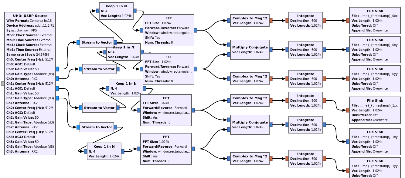
The flowgraph produces, for each of the two antennas, the power spectral densities \(E(|X|^2)\) and \(E(|Y|^2)\) and the cross product \(E(X\overline{Y})\). The averaging period is 0.1 seconds, and to make the flowgraph run in real time at 24.756 Msps I am only processing one out of every four FFT windows. This is something I am working on improving by using more FFT blocks in parallel to distribute the load accross more CPU cores.
The observations with this flowgraph were done around 2020-10-24 11:00 UTC. A total of four Gaileo and one GPS satellites were observed for a few minutes each. Antennas 1h and 4g were used with USRP0 and USRP1 respectively. The antennas were commanded manually and the flowgraph was stopped and started manually between the observations of each satellite.
LO d in the RFCB was used for both antennas and tuned to move 1575.42 MHz down to an IF of 512MHz. The USRPs were tuned to this IF as centre frequency. In the IF switch matrix an attenuation of 20dB was used, and the USRPs were set to a gain of 50dB (which was probably a bit high, in hindsight).
The analysis of the observations was done in this Jupyter notebook. To calibrate the polarization response of the system, I assumed a simple model with no polarization leakage or rotation, so that only gain and phase offsets between the X and Y channels need to be determined. Mathematically, we assume that\[\begin{pmatrix}e_x’\\e_y’\end{pmatrix} = \begin{pmatrix}g_x & 0\\0 & g_y\end{pmatrix} \begin{pmatrix}e_x\\ e_y\end{pmatrix},\]where \((e_x, e_y)^T\) is the Jones vector of the source, \((e_x’, e_y’)^T\) is the observed Jones vector, and the complex gains \(g_x\) and \(g_y\) need to be determined.
The complex gains can be found by assuming that the signal from a GNSS satellite is perfectly RHCP, so that the source Jones vector is \((1,-i)^T/\sqrt{2}\). In practice, I worked with Stokes parameters and calibrated the complex gains using the observations of the first satellite in order to have total intensity \(I = 1\) and so that all the polarized intensity was RHCP, which corresponds to the conditions \(Q = U = 0\) and \(V > 0\).
The main idea of this experiment was to verify how good this calibration stayed for other GNSS satellites in different parts of the sky. While GNSS navigation signals are nominally RHCP, the antennas are never perfect, and the axial ratio is slightly larger than one, and typically increases with the off-boresight angle. A satellite at the zenith is seen at zero off-boresight angle, while the off-boresight angle increases for satellites at lower elevations.
The figure below shows the polarization parameters obtained from the Stokes parameters for each of the satellites in the full 24.576 MHz measurement bandwidth. The horizontal axis represents UTC time in hours and minutes.
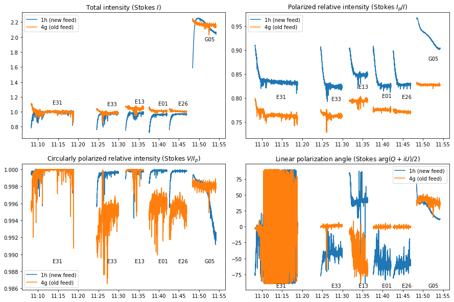
We see that the Galileo satellites have very similar total intensities, despite being at different elevations. The GPS satellite has approximately 3dB more power in this measurement bandwidth (to interpret this result, note that the sidelobes of the Galileo PRS signal are outside of the measurement bandwidth, so we are not observing the full Galileo E1 navigation signal). Only around 0.8 of the intensity is polarized. This is caused by the contribution of noise.
There is a strange effect that is convenient to comment. Note that at the start of the observation of each satellite the total intensity ramps up significantly over the course of one minute or so, while the fraction of polarized intensity ramps down. This happens because the total power increases, but the noise increases more than the signal, so the SNR decreases.
We have tried to track down how this effect happens and have found that it is produced by the USRP. We think that some of the LNAs slowly saturate in the presence of strong signals. The speed at which this happens suggests some thermal effect. We are testing how to adjust the gain properly to prevent these problems, and whether any strong out-of-band interferers might cause issues.
As we see in the plot of \(V/I_p\), more than 0.99 of the polarized intensity is RHCP. This means several things. First, that the GNSS satellite signals observed have less than 1% error from being perfect RHCP, since the calibration done with the observation of the first satellite stays good for the other ones. Second, that polarization leakage is small and can be ignored in many applications. In particular, this kind of calibration that only considers gain and phase offsets is appropriate for receiving circularly polarized signals by combining the complex voltages from the X and Y channels. This is important whe using ATA to observe satellites, as many use circular polarization.
The figure below shows the power spectral densities corresponding to the total intensity \(I\) and circularly polarized intensity \(|V|\) for each of the satellites. The values of \(I\) are shown with a strong line, while the values of \(|V|\) are shown with a semi-transparent line. We see how the noise biases the measurement of \(I\), filling in the spectral nulls of the modulations. These spectral nulls appear clearly in the measurement of \(|V|\), since the noise in the X and Y channels is mostly uncorrelated.
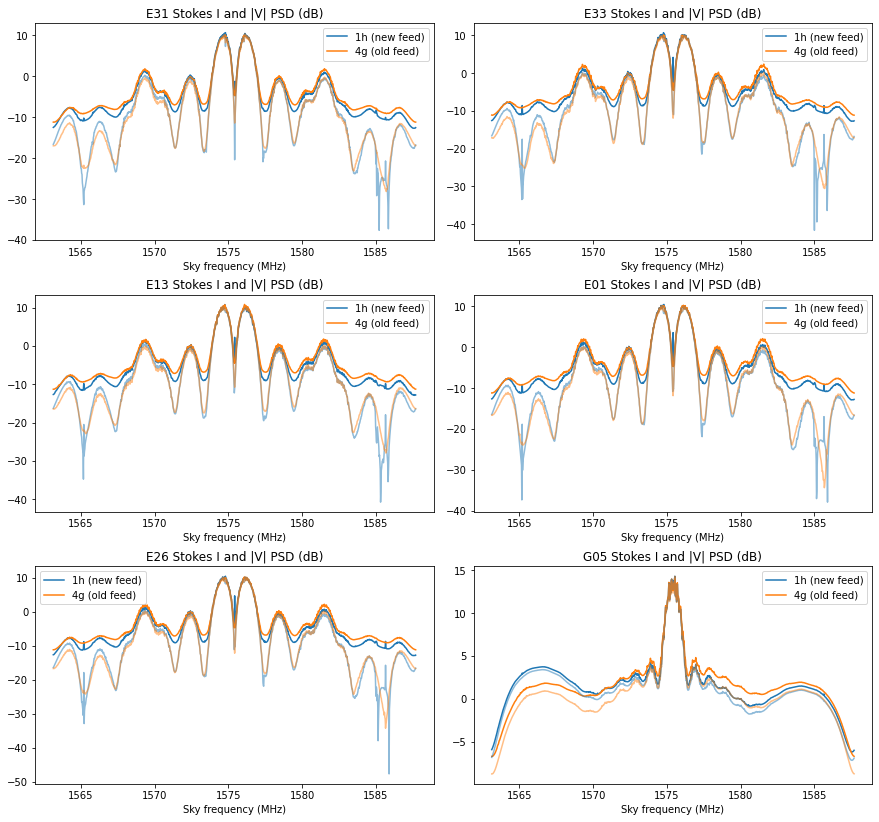
At the precision of around 1% that we are working with here, a single pair of complex gain coefficients \(g_x\) and \(g_y\) is valid for all the 24.5 MHz bandwidth. For larger bandwidths or higher precisions, it is necessary to take into account the frequency dependence of the calibration coefficients.
To improve my polarimetry experiments at ATA, I have read ATA Memo 87 and this paper about the Hamaker-Bregman-Sault Measurement Equation, which describes a model for the calibration of interferometric polarimetry. I’ve also been taking a look at the polarization calibration guidelines for VLA, and I’m looking forward to using astronomical sources such as 3C 286 for more precise calibrations.
One comment