Since the beginning of October, together with a group of people from the GNU Radio community, we are doing some experiments and tests remotely at Allen Telescope Array (ATA). This amazing opportunity forms part of the recent collaboration agreement between SETI Institute and GNU Radio. We are taking advantage of the fact that the ATA hardware is relatively unused on weekends, and putting it to good use for our experiments. One of the goal of these activities is to put in contact GNU Radio people and radio astronomy people, to learn from each other and discover what features of GNU Radio could benefit radio astronomy and SETI, particularly at the ATA.
I’m very grateful to Wael Farah, Alex Pollak, Steve Croft and Ellie White from ATA and SETI Institute for their support of this project and the very interesting conversations we’ve had, to Derek Kozel, who is Principal Investigator for GNU Radio at SETI, for organizing and supporting all this, and to the rest of my GNU Radio teammates for what’s being an excellent collaboration of ideas and sharing of resources.
From the work I’ve been doing at ATA, I already have several recordings and data, and also some studies and material that I’ll be publishing in the near future. Hopefully this post will be the first in a series of many.
Here I will speak about one of the first experiments I did at ATA, which is a recording of one Galileo GNSS satellite using two of the dishes from the array. This kind of recording can be used to perform interferometry. GNSS satellites are good test targets because they have strong wideband signals and their location is known precisely. The IQ recording described in this post is published as the dataset “Allen Telescope Array Galileo E31 RF recording with 2 antennas and 2 polarizations” in Zenodo.
An overview paper describing the characteristics of ATA can be found here. The interested reader can find more information in the reading list from the GNU Radio hackathon and in the ATA memo series.
The recording is a short 15 second recording of Galileo satellite E31. Antennas 1h and 4g were used for this recording. As all the ATA antennas, these are 6m dishes with a Gregorian subreflector and log-periodic feed. Antenna 1h has one of the new feeds, which covers 0.9-14 GHz and is described in this article, while antenna 4g has one of the old feeds, covering 0.5-10 GHz. The two antennas give a baseline of 242 metres.
The signals from the antennas are downconverted by the RFCB, which for this recording was configured to mix the frequency of 1475.42 MHz down to an intermediate frequency of 629 MHz. The same local oscillator D is used to downconvert both antennas and polarizations.
The IF is sampled by two USRP N32x. The two channels of each of them are used to sample the two polarizations (X and Y) from a single antenna. They are connected to a 10 MHz external reference and PPS signal coming from the observatory time and frequency distribution system. LO sharing was not used for this recording, so there is a random phase offset between each of the channels. A sample rate of 30.72 Msps was used to prevent losing samples. Recording the four channels to disk at higher sample rates is something that we are currently improving. Since the centre frequency is 1475.42 MHz, this is enough to capture the full E1BC Open Service CBOC modulation and part of the E1A PRS BOCcos(15, 2.5) sidebands.
I have started a Github repository to put the Jupyter notebooks I’m doing for my work at ATA. The repository is called ata_notebooks and it is quite similar in spirit to my jupyter_notebooks repository (though I will try to keep it more tidy). The Jupyter notebook for my analysis of this recording can be found here. In that notebook, Dask is used to implement an FX correlator, and then I do basically everything I could think of with the correlations.
Here I will give an overview of the results. I won’t go into much detail, since the calculations are already described in the notebook. The figure below shows the power spectral density of each of the channels. Note that each of the channels has slightly different gain, and also different SNR, which can be observed by the depth of the signal nulls.

Another thing that is interesting to mention is the fact that the CBOC signal looks noisy, because it has spectral lines caused by the periodic PRN codes, while the PRS sidebands look smooth, because they are an encrypted signal.
Since the recording is short, it is possible to approximate the baseline delay rate by a constant. Thus, we are able to determine an initial baseline delay of 184.368 m and a delay rate of -0.024052 m/s. Note that the baseline delay includes both the geometric delay between the antennas and also instrumental delays. For example, the runs of optical fibre used by the two antennas to route the signal to the signal processing room have different lengths.
Using these corrections we can maximize the correlation power by accumulating over all the frequency bins and stop the fringe rotation to accumulate coherently over all the recording. Therefore, the products from this observation are complex visibilities for the whole frequency band, and complex visibilities over frequency. Since the signal is strong, there is enough SNR in the complex visibilities over frequency to see instrumental frequency-dependent effects in the passband.
Since the Galileo signal is nominally RHCP, we would expect to see the same amplitude and a phase offset of 90º in the two linear X and Y polarizations for the same antenna. Zero-baselines formed by the channels 1hx-1hy and 4gx-4gy, as well as the cross-polarization baselines 1hx-4gy and 1hy-4gx are included in the study.
The visibilities are calibrated in the following manner. We assume that the same signal plus noise power should be present in all the channels. This is used to calibrate in amplitude. For phase calibration, we phase-reference all the channels to 1hx, multiplying each of the other channels by a complex number of modulus one such that the visibilities for each of the baselines involving 1hx are real and positive.
The visibility phase across frequency is quite interesting, as it shows frequency dependent instrumental phase delays in the passband. The spikes that appear at regular frequency spacings correspond to the signal nulls, where the visibility amplitude drops down. Other than this, each of the visibility phases traces a smooth curve according to different phase delays in each of the channels. These delays would need to be calibrated out.
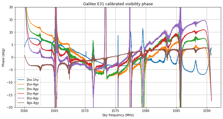
The phase closures are also very interesting. They should be zero regardless of phase delay calibration. However, we see that there are some deviations from zero in some of the closures, particularly those involving 1hx-1hy. I’m not sure what this means. Note that this effect happens above 1580 MHz, and there is also something strange going on with the PSD of 1hx and 1hy above 1580 MHz. It has a few dB’s less than it should, so the PSD doesn’t look completely symmetric.

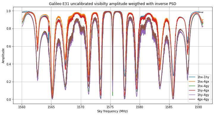
The next figure perhaps needs some explanation. Here we take, for each frequency bin, the visibility amplitude and divide it by the geometric mean of the power in that bin of the two signals in that baseline. By doing this we get a number between zero and one that indicates which fraction of the signal power has ended up in the correlation. The main lobes of the CBOC signal and the PRS sidebands show values very close to one, since they have a very strong SNR. The other parts of the signal show smaller values, since they correspond to weaker sidelobes with less SNR. The effect is especially marked for baselines involving 4gy, because that channel has overall less SNR for some unknown reason.
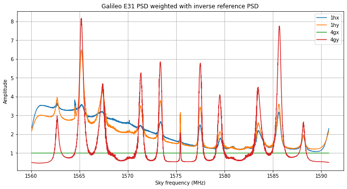
To characterize the amplitude over frequency behaviour of the receive chain, we take the PSD of channel 4gx as a reference, since that channel has the best SNR. Then we can plot the PSD of each channel divided by the PSD of channel 4gx. Channels 1hx and 1hy show a sloping behaviour which we had already noted in the asymmetry of their PSD plots.
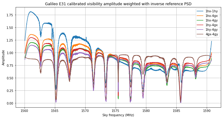
In the same manner, we can divide the visibility amplitudes by the PSD of 4gx. We see the same sloping behaviour in the baselines that involve 1hx or 1hy.
In addition to studying the complex visibilities, I have also compared the baseline delay rate as measured by the interferometric observation with a calculation using SP3 files describing the satellite positions. This calculation is sensitive to the baseline vector, but we haven’t measured the baseline accurately yet. I have used the coordinates that come from looking at the dishes in Google maps satellite view, so they are accurate to a metre or so. We are working on measuring the baseline more accurately by using long interferometric observations of astronomical sources.
The C code that computes the delay rate can be found in the repository. It uses RTKLIB for the calculations and includes a run.sh script that calls it with the appropriate parameters. This code gives a delay rate of -0.024043 m/s. The difference between this and the delay rate measured by the interferometric observation is on the order of 10 um/s. This is within the error budget for this interferometric measurement.
This observation serves as a proof of concept to show what can be achieved with interferometric observations of GNSS satellites and how the calculations can be done. The visibilities over frequency have shown small differences in phase and gain between each of the four channels. These should be calibrated out for more serious observations. Astronomical continuum sources are a good source for this calibration since they are spectrally flat.
Hello Dr Estevez
Would you mind letting me know what gnuradio .grc file you have used to record the 4 channels in a time-synchronized way?
Hi John,
Thanks for the question. I have added this flowgraph to the repository. It’s not exactly the same one that was used in this recording, but it is very similar and it is what I’m using now for other recordings.