Earlier this year, I published a post showing our results of the interferometric imaging of Cassiopeia A and Cygnus A at 4.9 GHz with the Allen Telescope Array. Near the end of July, I decided to perform more interferometric observations of Cygnus A at a higher frequency, in order to obtain better resolution. I chose a frequency of 8.45 GHz because it is usually a band clean of interference (since it is allocated to deep space communications), it is used by other radio observatories, so flux densities can be compared directly with previous results, and because going higher up in frequency the sensitivity of the old feeds at ATA starts to decrease.
This post is a summary of the observations and results. The code and data is included at the end of the post.
Observation set up
For these observations, I used 6 antennas that have recently entered into service. The configuration of the USRPs is the same as I described in my post from March, so only one baseline can be correlated at a time and the set of baselines that can be formed is limited to those obtained by choosing one of the antennas available for USRP1 and one of the antennas available for USRP2, as follows:
- USRP1: 2c, 2e, 3l, 5b
- USRP2: 2j, 2m
Therefore, only 8 baselines can be formed with these 6 antennas.
The sources observed in these observations are as follows:
- 3C286 as polarization calibrator, flux density scale calibrator, and backup phase calibrator
- J2007+404 as primary phase calibrator; this is a 2.85 Jy source listed as a VLA calibrator
- 3C84 as bandpass calibrator and backup phase calibrator
- Cygnus A as science target
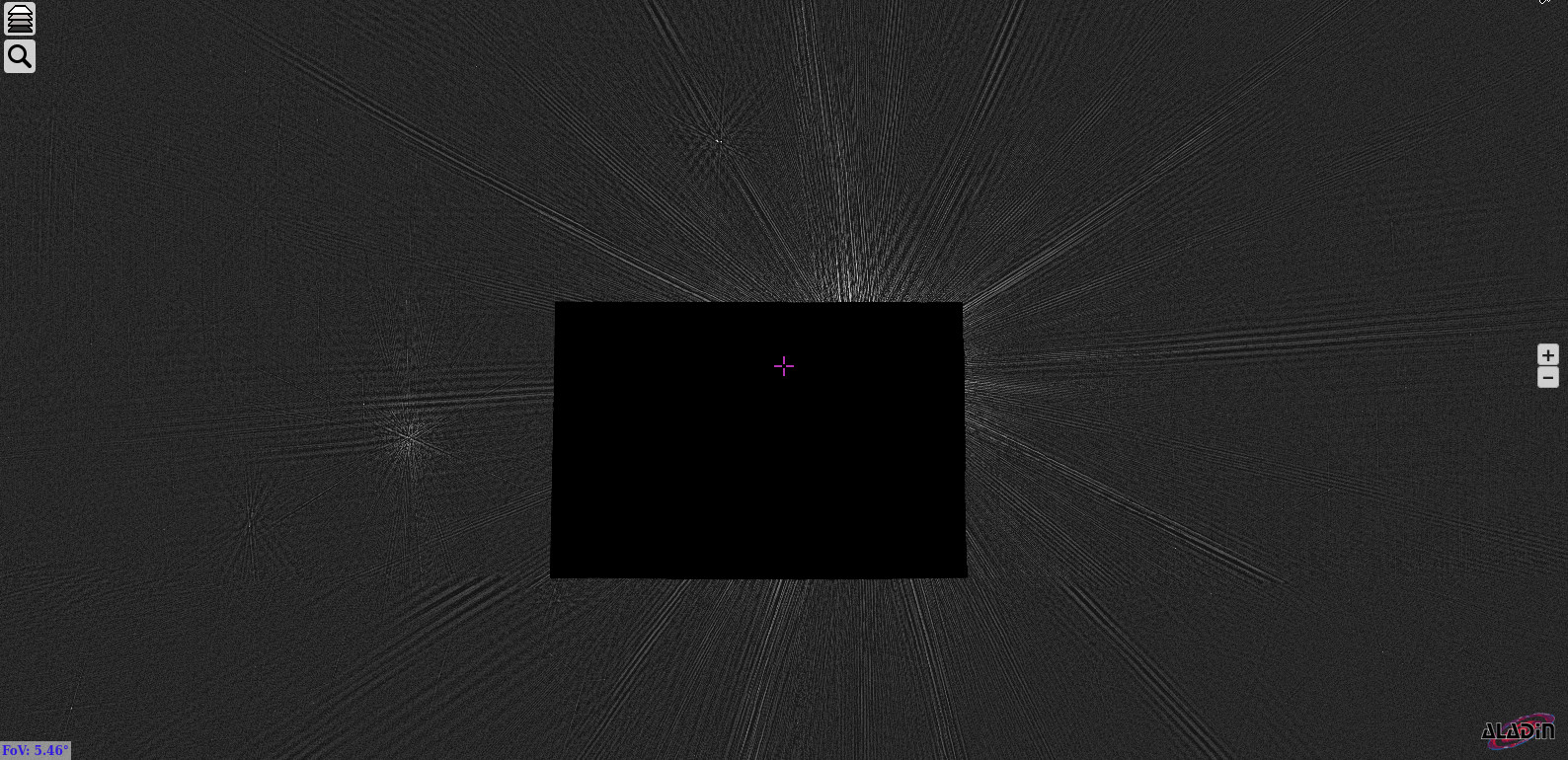
Cygnus A is located at only 1.59 degrees separation from the calibrator J2007+404. The image below, taken from the VLASS 2-4 GHz VLA sky survey shows both of them. Cygnus A is inside the black box, since VLASS excludes very strong sources, and J2007+404 can be seen towards the left of Cygnus A, showing large sidelobes in this quicklook image due to its rather high flux density (compared with the sensitivity of this survey). This image has been obtained with the web interface to the VLASS2.1 HiPS data, which allows us to explore the radio sky easily.
I used the same GNU Radio software correlator as back in March. This is contained in the ata_interferometry Github repository. The observed bandwidth was 40.96 MHz, using the X and Y polarizations. All the polarimetric autocorrelations and cross-correlations were computed in real time, and phased in post-processing and reduced to UVFITS files with 64 frequency channels and 1 second integration time.
Observation scheduling
The observations were carried out during three consecutive days: 23, 24 an 25 July. The first day was a full track observation of 3C286 only. The goal of this observation was to gather as much data as possible for polarization calibration, and additionally to serve as a check of the system.
The second day, the observation of all the targets was carried out, following this order:
- 3C286 was observed as soon as it rose, and until Cygnus A rose
- When Cygnus A and J2007+404 rose, they were scanned alternatively, with infrequent scans of 3C286
- When 3C84 rose, the pattern of scanning Cygnus A and J2007+404 continued, but the infrequent scans of 3C286 were replaced by infrequent scans of 3C84
- When Cygnus A and J2007+404 set, 3C84 was observed for an hour more, with the goal of using this final segment for bandpass calibration
Unfortunately, there was a problem with the observation script throughout the night, before Cygnus A rose, so several hours of data were lost. The third day the same schedule was followed, with the observation script already corrected, so all the data was gathered.
The figure below shows the calibrated visibility amplitudes of the whole three days. Colouring is by field, with 3C286 in black, J2007+404 in pink, Cygnus A in orange, and 3C84 in green.
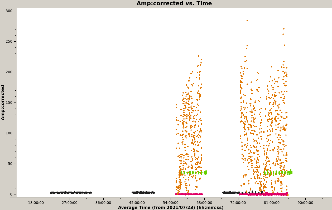
The plot shows the great differences in brightness of the sources, with Cygnus A being by far the brightest. It is often not easy to get calibrators close to the science target that have a flux density of at least a few Jy, which is necessary for good results with the ATA 6.1 m dishes observing with only 40 MHz of bandwidth and one baseline at a time. Therefore, the presence of J2007+404 so close to Cygnus A is a happy coincidence.
3C84 is by far one of the strongest compact calibrators, so it is quite useful for bandpass calibration and other calibrations that benefit from high SNR.
Calibration
Calibration and imaging was performed in CASA 6.2.0. First, some flagging of interference was done with tfcrop. Then data that was visibly bad when examining the amplitudes or phases with msview was manually flagged.
Two separated bandpass calibrations were performed using the scans of 3C84 at the end of the second and third day, after Cygnus A had set. The calibration from the second day turned out to be much better because there was some unknown problem during the third day that caused a loss in sensitivity. The amplitude of the cross-correlations decreased suddenly, while the amplitude of the autocorrelations wasn’t affected. Moreover, the variance of the visibilities increased significantly. Therefore, the bandpass solution from the second day was chosen to be applied to all the data.
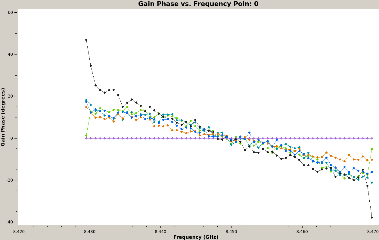
The figures below show the bandpass solutions. As I remarked in my post from March, it is not possible to use CASA for a delay calibration because of the baseline-by-baseline scans. Therefore, the delays, which are small, are absorbed by the bandpass phase.
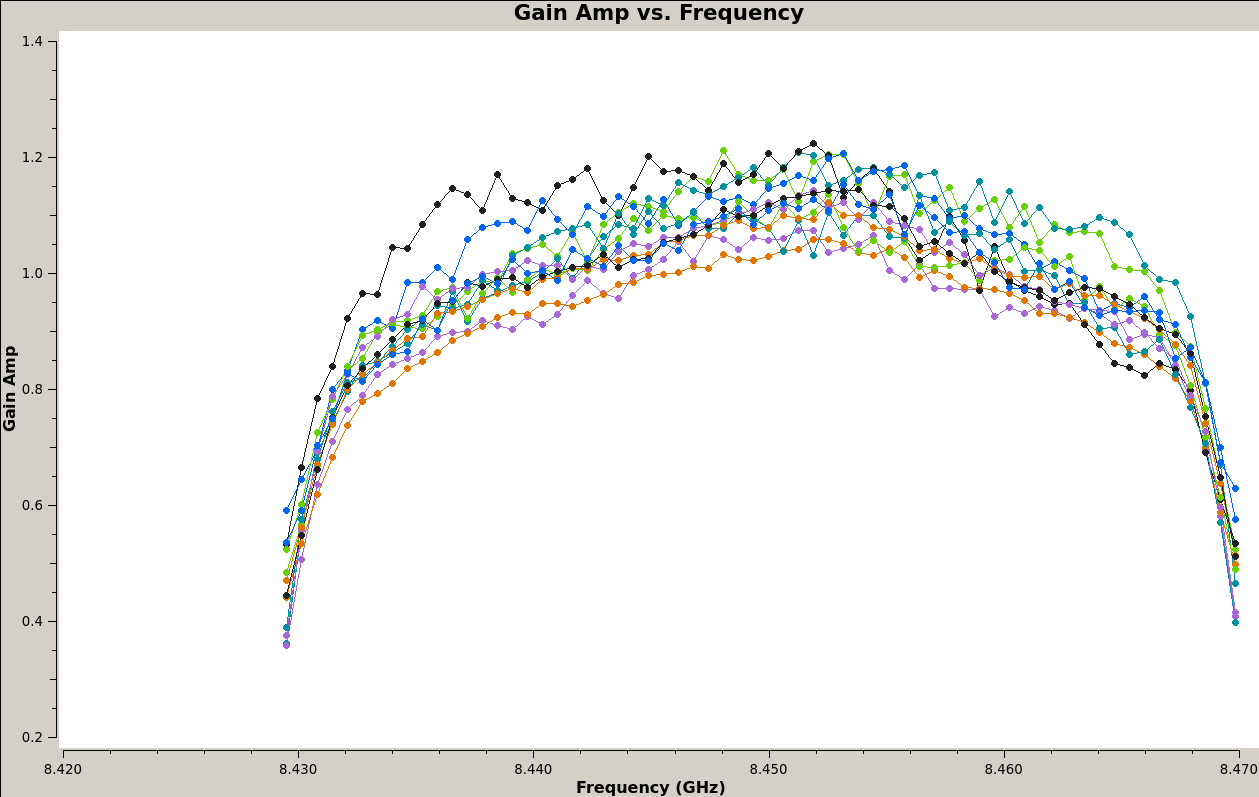
It is interesting that the reference antenna, 2j, has a noticeable delay difference in the X and Y polarizations, whereas the rest of the antennas have more similar delays.
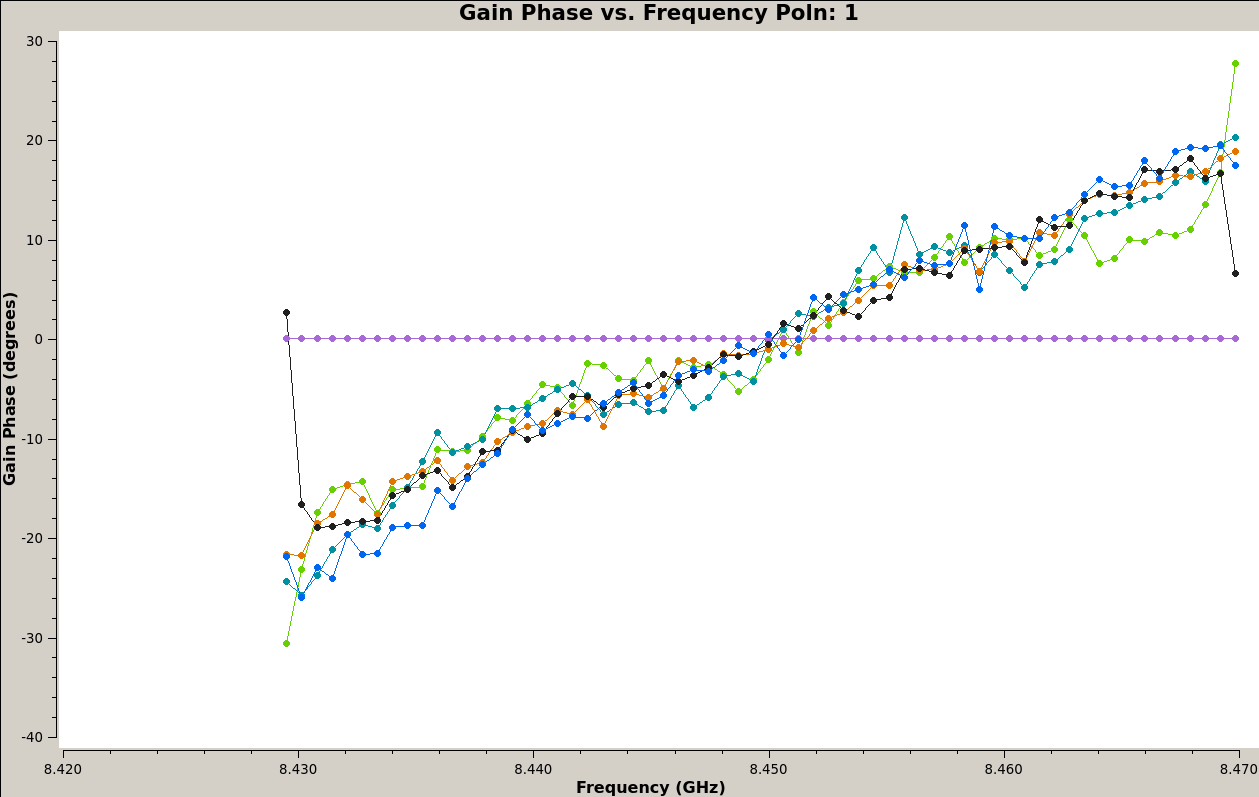
Besides calibrating the bandpass, these scans of 3C84 are used to perform a time-independent phase calibration, which is then used as the phase offset between the X and Y polarizations. This allows all further phase calibrations to be performed in a polarization-independent way, which increases the SNR.
Next, a polarization-independent phase calibration is done on each compact calibrator. The solution intervals are chosen manually during most of the observations in order to fit well with the 8 baseline cycle.
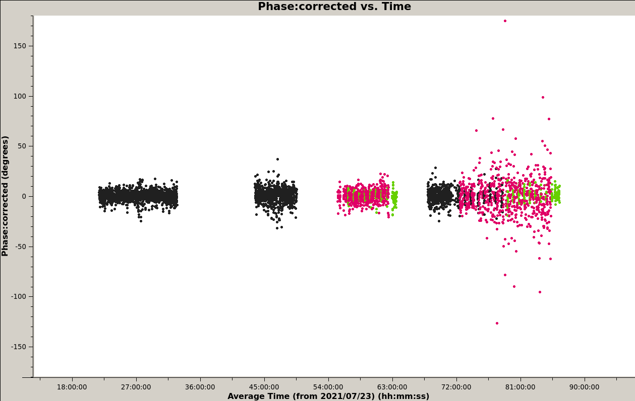
The figure below shows the results of applying this phase calibration, together with the bandpass and X-Y phase offset to the three compact sources 3C286 (black), J2007+404 (pink) and 3C84 (green). The decrease in sensitivity at some point during the third day is apparent in the noise in the phase of J2007+404.
After phase calibration, amplitude calibration is done. This is carried out in a polarization-dependent way, since the gains of the two channels can change independently. The idea is to use 3C286 as the flux density calibrator and to transfer the flux scale to the other calibrators. However, there are the following two quirks to handle.
On the second day there is a long gap without data, separating 3C286 and the other sources. This means that the amplitude scale from 3C286 can’t be transferred to the other sources, since the gains can have changed somewhat during that gap (and in fact the correct amplitude transfer shows that it has changed). Therefore, what we do for this day is to use 3C84 as the amplitude scale, forcing the flux measured on the third day during calibration.
On the third day we have the problem with the change in sensitivity, that causes a sudden decrease of visibility amplitudes. The segments before and after the change are calibrated and transferred separately, and this seems to work well.
The figures below show the calibrated amplitudes of each of the calibrators. There is perhaps a slight difference in amplitude for 3C84 comparing the second and third days. This is caused by the peculiar calibration process explained above, but it is something minor.
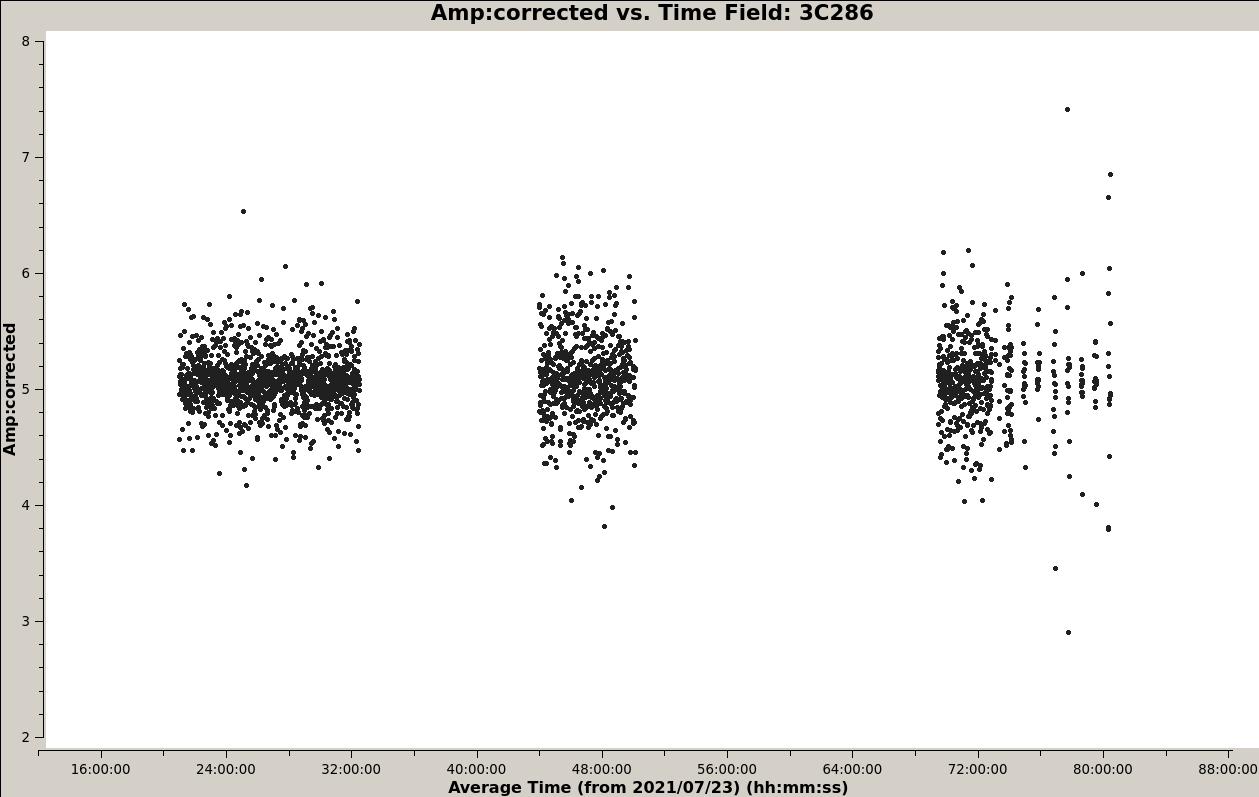
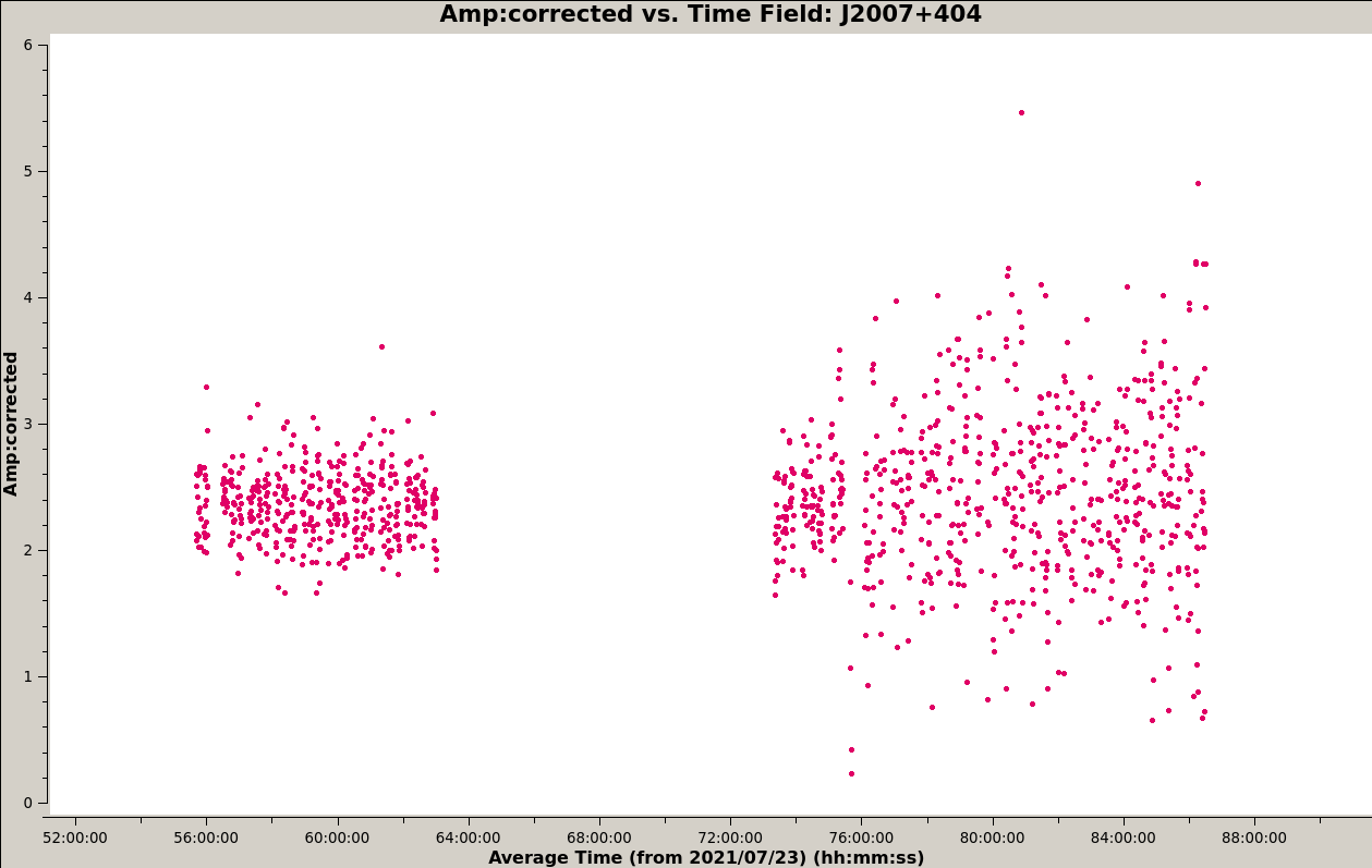

For each of these sources, the bandpass and X-Y phase offset from 3C84 on the second day and the amplitude and phase calibration from itself are used. For Cygnus A, the bandpass and X-Y phase offset are also taken from 3C84 and the amplitude and phase calibration is taken from J2007+404.
Imaging
Imaging is done using multi-scale cleaning and roughly the same parameters as in my post from March. A pixel size of 4 arcseconds is used. In contrast to that post, an image size of 512×512 pixels is used to image the whole primary beam, though we don’t expect to see any other objects away from the phase centre in each field.
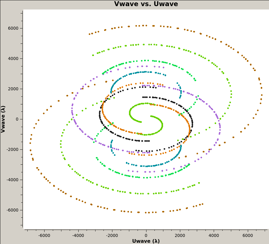
The figure below shows the UV coverage for Cygnus A. There is coverage between approximately 0.2kλ to 7λ, which corresponds to resolutions between 30 arcsec and 17 arcmin.
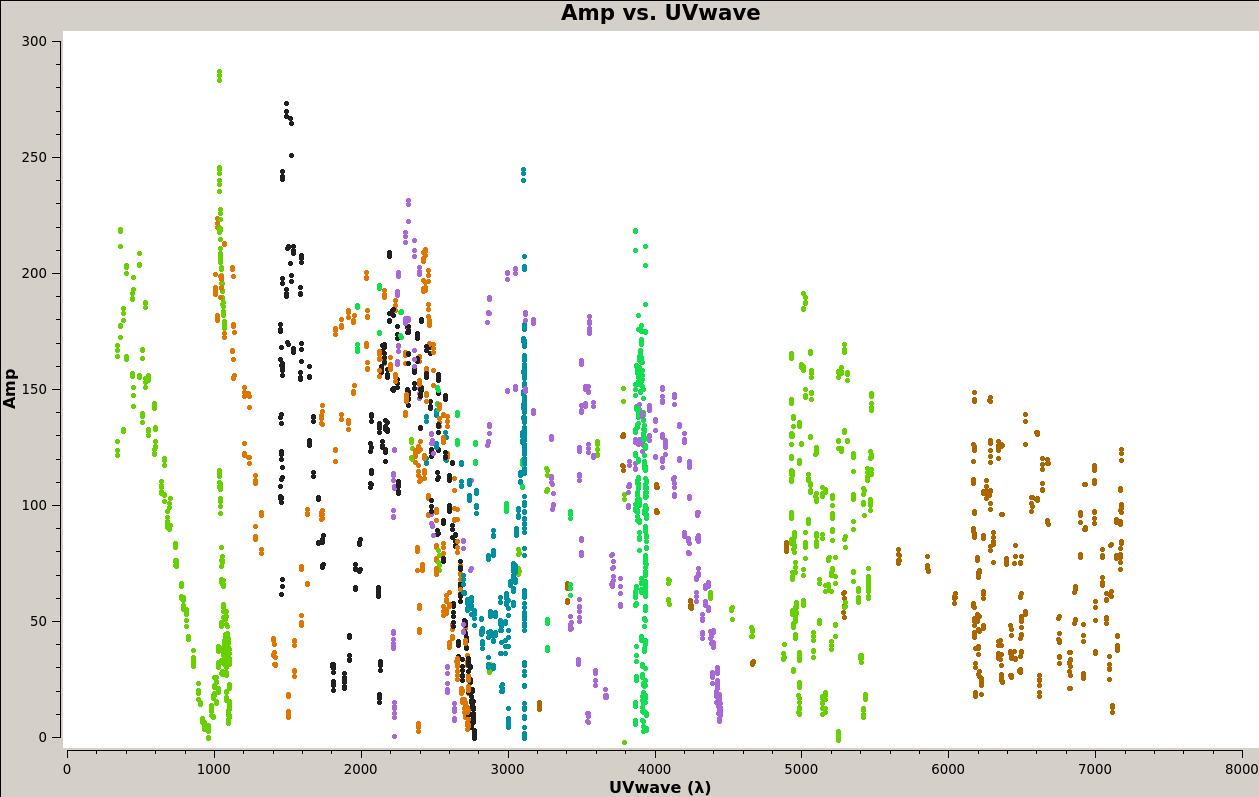
The next figure shows the amplitude versus modulus of (U,V). We can see that several baselines are probing the first nulls of the visibility of Cygnus A. In some of the baselines we see that the line is double. There are somewhat different gain calibrations on each of the two days. This will be fixed with self-calibration after imaging.
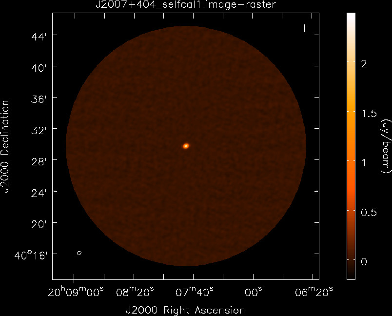
For the compact sources, first an image is done without many clean iterations to generate a model, then phase and amplitude self-calibration is made, and a second image is cleaned with more iterations. The images are not very interesting, since the sources are unresolved, but imaging is a good way to check that everything is working correctly.
For Cygnus A, first an image is cleaned, then a phase self-calibration is done, a new clean image is done, and finally a phase and amplitude self-calibration is done with the new image, thus producing a final self-calibrated image.
The SNR for each of the images is shown below. This is computed as the quotient of the maximum pixel brightness and the RMS in an area that does not contain the object. We can see how the SNRs of 3C84 and Cygnus A increase greatly after self-calibration. Since these objects are very bright, the image SNR is mainly limited by calibration errors.
3C84.image SNR: 163.43
3C84_selfcal1.image SNR: 406.75
3C286.image SNR: 409.76
3C286_selfcal1.image SNR: 474.12
J2007+404.image SNR: 182.80
J2007+404_selfcal1.image SNR: 189.06
CygA.image SNR: 168.43
CygA_selfcal1.image SNR: 230.08
CygA_selfcal2.image SNR: 539.46
The images for the three calibrators are shown below.


The next figure shows the image for Cygnus A. We can clearly see the double source structure.

A zoom to this image and the addition of a contour plot reveal more detail. The contours are set at 2.5, 5, 10, 20, 30, 40, 50, 60, 70, 80 and 90% levels.
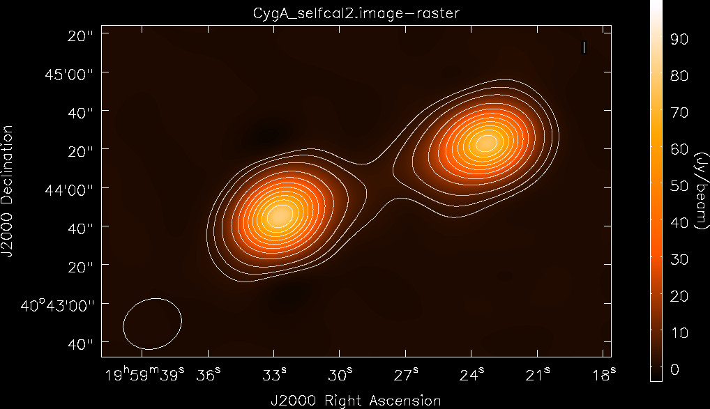
In the central part between the two lobes there is a flux of around 3 Jy/beam. This is significantly higher than the noise floor, which is a fraction of a Jy/beam. It provides evidence that we are detecting the small central component, that corresponds to the supermassive black hole in the active galaxy. The figure below, taken from this page, shows an image done with VLA at 5 GHz that has 60 times more resolution and shows the central component clearly.
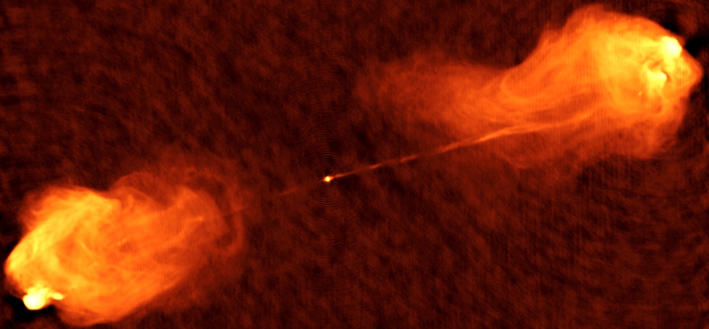
The total flux density in the image of Cygnus A is 201.6 Jy, and the maximum brightness is 79.7 Jy/beam.
Polarimetry
I hoped to use these observations to study the polarization of Cygnus A. This is the reason why the first day was devoted to a full track observation of 3C286. However, I have not been able to obtain a satisfactory polarization calibration. It is difficult to detect the polarized signature in the cross-hands due to the large leakages and low SNR. Moreover, the changes in the relative amplitudes of the parallel-hands do not seem so consistent between different baselines, for some unknown reason.
I have even been following the CASA tutorial for polarimetric imaging of 3C286 with ALMA (since ALMA also uses a linear polarization basis, unlike the VLA), trying to improve my techniques. However, after trying to do something with the data for a while, I think that it is not good enough, and better data needs to be gathered.
Code and data
The code used in this post for correlation and phasing is the usual GNU Radio FX software correlator pipeline from the ata_interferometry repository. The calibration and imaging in CASA was done with this script.
The data has been published as the dataset “Cygnus A 8.45 GHz interferometric observation with Allen Telescope Array” in Zenodo.
This is very interesting work. Congratulations on your results and thank you for sharing them