Over the last few weeks I have been helping the Allen Telescope Array by calibrating the pointing of some of the recently upgraded antennas using the GNU Radio backend, which consists of two USRP N32x devices that are connected to the IF output of the RFCB downconverter. For this calibration, GPS satellites are used, since they are very bright, cover most of the sky, and have precise ephemerides.
The calibration procedure is described in this memo. Essentially, it involves pointing at a few points that describe a cross in elevation and cross-elevation coordinates and which is centred at the position of the GPS satellite. Power measurements are taken at each of these points and a Gaussian is fitted to compute the pointing error.
The script I am using is based on this script for the CASPER SNAP boards, with a few modifications to use my GNU Radio polarimetric correlator, which uses the USRPs and a software FX correlator that computes the crosscorrelations and autocorrelations of the two polarizations of two antennas. For the pointing calibration, only the autocorrelations are used to measure Stokes I, but all the correlations are saved to disk, which allows later analysis.
In this post I analyse the single-dish polarimetric spectra of the GPS satellites we have observed during some of these calibrations.
Observation set up
Antennas 5b and 2j were used to collect the data used in this post. The observations were done between June 2 and 4. The USRPs ran at an IQ sample rate of 40.96 Msps. Each scan has a duration of 20 seconds. As usual in the pointing calibration with GPS satellites, to prevent saturation the PAMs of the feeds were set to a fixed attenuation of 27 dB.
The USRPs used a gain of 45 dB, which gives a good increase in the noise floor of 10 to 20 dB when the IF output is connected to the USRP. The USRPs shared a common LO, 10 MHz and 1PPS reference. The USRP N321 was used to digitize both polarizations from antenna 5b, and the USRP N320 was used for both polarizations of antenna 2j. The software FX correlator was configured to use 2048 FFT bins.
Data selection
The data is clustered according to the GPS satellite observed and the timestamp, in order to group together all the measurements that the pointing calibration script performs with a satellite before moving to another satellite. Each scan is averaged in time.
The total power in the X polarization of antenna 5b is used to select the strongest scan for each group, since that will give the pointing where the satellite is closest to the beam centre. That scan is used as representative of that satellite at that observation time, the rest of the scans are discarded.
Calibration
In the polarimetric calibration, only the amplitude gains and the X-Y phase offsets are found. Polarization leakage is not taken into account. To perform the calibration, the data from all the satellites and timestamps that were selected in the previous step is averaged. It is assumed that this yields a signal that is perfectly RHCP across all the spectrum.
First a frequency independent calibration is done on the average of the central half of the spectrum. The amplitude gains are found from the XX and YY correlations, and the phase offset is found from the XY* correlation. Using this frequency independent calibration, the Stokes I PSD is found by applying the calibration and averaging the two antennas and polarizations.
Then a frequency dependent calibration is done. Since the PSD of the GPS signal is not flat, the correlations are first divided by the Stokes I PSD computed in the previous step. This is the final calibration. Note that this calibration procedure is able to estimate the X-Y phase offsets across the full passband. However, it is not able to estimate that gain of the passband, because we do not have an absolute reference for the PSD of the GPS signals. It is only able to estimate gain differences between each of the channels.
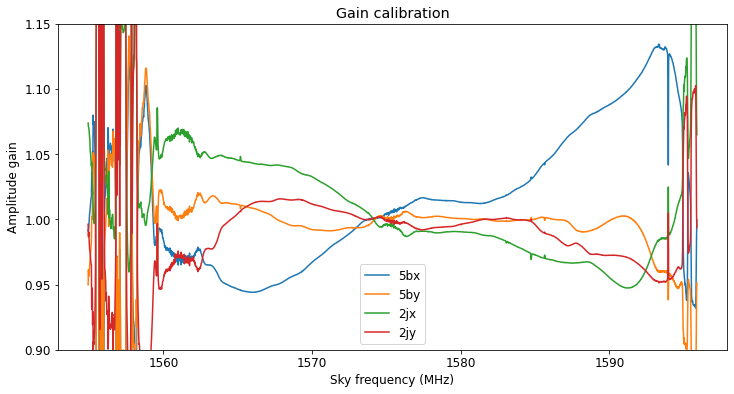
The results of the calibration are plotted below. Regarding the gain we can see that the difference between each of the four channels changes only around 5 to 10%.
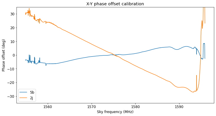
Regarding the phase offset we see that antenna 2j has a large phase versus frequency slope. The total phase difference of some 60 degrees across 40.96 MHz of bandwidth corresponds to a delay of around 4 ns.
Results
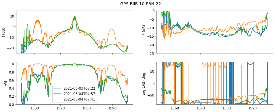
The polarimetric spectra of each GPS satellite, obtained from the average of the two antennas, is plotted in four panels as shown in the figure below. Each of the observations of the satellite is plotted in a different colour.
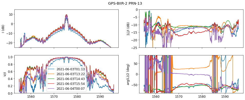
The upper left panel shows Stokes I. The lower left panel shows the degree of RHCP in linear units. This is computed as -V/I (we use the convention that V is negative for RHCP). We expect that this value is very close to one except when the signal is weaker, since noise contributes to I but not to V.
The upper right panel shows the degree of linear polarization in dB units. We typically get values between -20 and -10 dB. The presence of linear polarization is both due to leakage in the ATA feeds and to the RHCP polarization of the satellite not being perfect (it will typically degrade for satellites at lower elevation, since the antenna is seen at a higher boresight angle). The lower right panel shows the angle of the linear polarization.
We see that the same satellite presents different linear polarizations (in particular the angles are significantly different) at different times. This seems to indicate that at least some amount of this linear polarization that we are measuring is not an instrumental effect, but due to the satellite.
It is interesting to see how the spectrum of the satellites of the different blocks (generations) differ, due to the presence of new signals in the newer blocks and to different power sharing between the signals. To understand the GPS signals, it the figure below is useful.
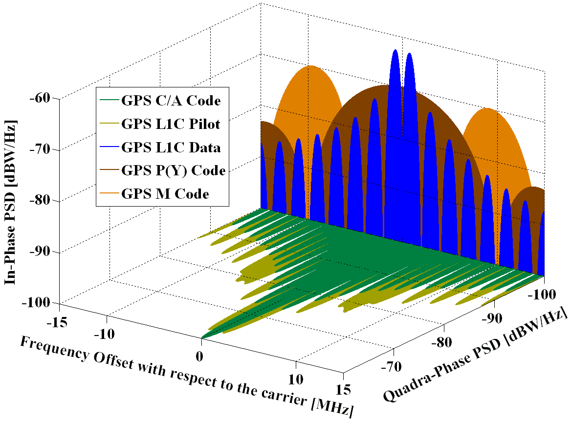
The satellite shown above, PRN-13, is a good example of the oldest block in operation, BIIR, which only uses the C/A and P(Y) code signals.
The next block is BIIRM, which introduces the M code signal. The modulation of this signal is BOC(10, 5), so it should appear in the nulls of the BPSK(10) modulation of the P(Y) code. However, we see nothing like that in the spectrum of any of the BIIRM satellites (PRN-15 below gives a good example). We only see BPSK(10) and BPSK(1) modulations, as with the BIIR satellites. The difference, however, is that the relative power of the BPSK(10) modulation is much higher for the BIIRM satellites in comparison to the BIIR satellites. This is clear from the fact that the BPSK(10) modulation in the plot below hides most of the sidelobes of the BPSK(1) modulation.
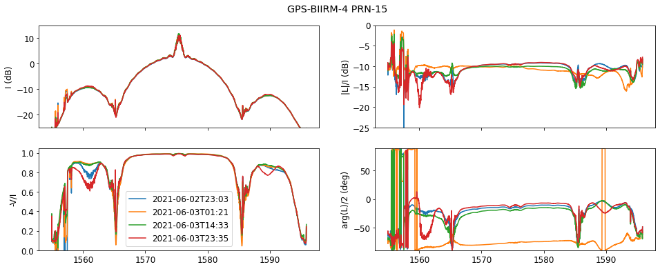
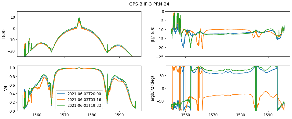
The lack of the M code signal is interesting. It also happens with the BIIF satellites, whose spectrum is very similar to the BIIRM satellites.
Finally, we have the new BIII satellites. These introduce the L1C TMBOC modulation. Interestingly, the BIII satellites do transmit the BOC(10, 5) M code signal.
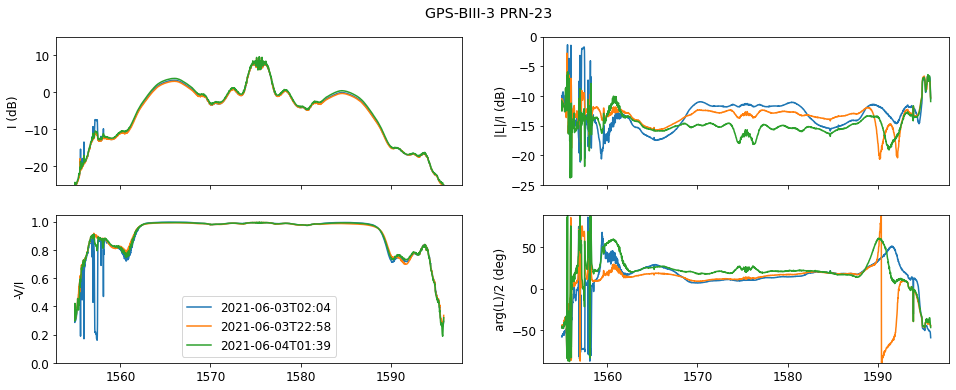
Something interesting is the amount of variability in the power of the M code signal. The satellite shown above does not display this effect, but the other BIII satellites do. The plot of PRN-14, the newest GPS satellite gives a good example. Note that the difference of the power in the M code signal in the four observations is much larger than in the rest of the spectrum.
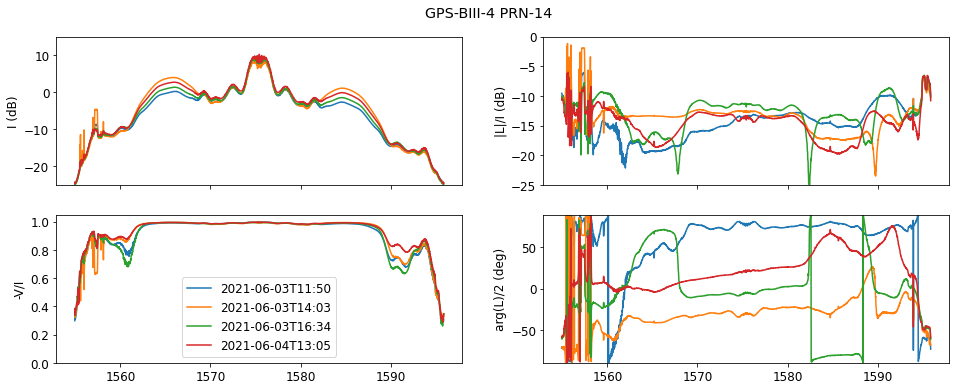
Another interesting aspect regarding the M code signal is that in some observations it seems to have a substantially different linear polarization from the rest of the spectrum. For instance, see the green trace in the figure above. It is known that the BIII satellites have a high-gain spot beam antenna to broadcast the M code, in addition to the usual wide-angle antenna that covers the full Earth. The changes in linear polarization might be caused by this, but it is difficult to get any quantitative measurements, since we have not calibrated instrumental effects properly.
Many of the satellites show spectral lines in the nulls of the P(Y) BPSK(10) modulation, at 10.23 MHz from the centre frequency. This can be seen in several of the figures shown above. I do not know the cause of this.
Some of the observations show unexpected signals from other GNSS satellites that happened to be in the antenna beam by chance. The blue trace for PRN-21 shows a Galileo satellite. The fact that the signal of the GPS satellite is absent can be explained because some of the pointing calibration measurements are taken with the satellite outside the beam, in order to measure the noise floor for the Gaussian fit. In this case, a Galileo satellite happened to be in the position of the noise floor measurement, and was selected in the process described above, where the only the strongest scan of each observation is taken into account.

This Galileo signal serves to illustrate a property of the GNSS signals’ spectra. GNSS signals that have periodic codes have spectral lines, which causes their spectrum to appear a bit fuzzy, as it happens to the spectrum of the CBOC Galileo Open ervice signal in the centre of the spectrum. In contrast, aperiodic cryptographic signals do not have spectral lines, so their spectrum looks completely smooth. This happens with the sideband of the Galileo PRS BOCcos(15, 2.5) modulation at the sides of the spectrum.
A similar signal appears in one of the observations of PRN-22, but this is actually the signal of a Beidou-3 satellite. The easiest way to notice the difference between Galileo and Beidou-3 satellites is that the left sideband of a Beidou-3 signal looks fuzzy, because of the B1I open signal (which is a BPSK(2)). Additionally, the B1A encrypted modulation is BOC(14, 2), so its sidebands are a bit narrower and closer to the centre than those of Galileo PRS.
Data and code
The calculations and plots shown in this post have been done in a Jupyter notebook, which can be downloaded here. This includes plots for 30 different GPS satellites.
The raw data from the FX correlator output is too large for sharing conveniently, since it is sampled in time at a rate of 10 Hz. The time averaged spectra have a more manageable size and are included in the same repository as a Python pickled file. This allows re-running the notebook and reproducing the results.