Bill Gray, from Project Pluto is doing a great job trying to estimate the orbit of Chang’e 5 as it travels to somewhere around the Sun-Earth L1 Lagrange point (see my previous post). He is using RF pointing data from Amateur observers and the Allen Telescope Array, since the low elongation and the distance of the spacecraft have made it impossible to observe it optically.
For this task, the pointing data I am obtaining with my observations on Allen Telescope Array as part of the activities of the GNU Radio community there is quite valuable, since the 6.1 metre dishes give more accurate pointing measurements than the smaller dishes of Amateurs. The pointing data from ATA should be accurate to within 0.1 or 0.2 degrees.
To try to get more accurate data for Bill, last weekend I decided to do a recording with two dishes from the array, with the goal of using interferometry to obtain a much more precise pointing solution that what can be achieved with a single dish. This post is a report of the processing of the interferometric data.
The recording was done with dishes 2h and 4g, which span a baseline of 176 metres. As usual, the 8471.2 MHz and 8486.2 MHz telemetry signals from the spacecraft were recorded using 480ksps IQ slices. On both days I tried to record for all the time that the spacecraft was in view.
On Saturday 26 I made a mistake with the conversion between local time and UTC and unfortunately I started the observation one hour and 30 minutes late. On Sunday 27 I managed to record for almost all the time that the spacecraft was in view. Luckily the script I described in my previous post to sweep a map of the sky and find the signal worked quite well and I could found the signal quite fast both days.
After Chang’e 5 set below 16.8 degrees each day, I followed with an interferometric observation of the quasar 3C286 in case it was needed for calibration. I also needed to observe several astronomical sources in order to determine the 2h-4g baseline accurately, so I did those while Chang’e 5 was not in view. In a future post I will describe the procedure I use to compute the baselines, which so far I’ve used to successfully solve for 1a-4g and 2h-4g at 8.4 GHz.
The IQ recordings of the Chang’e 5 telemetry signal are processed with this GNU Radio flowgraph, which processes each antenna and polarization separately, uses a PLL to lock to the residual carrier of the signal, and writes phase measurements to a file at a rate of 10 Hz. The phase measurements for the two antennas are then subtracted to obtain the interferometric visibility phase. Note that since the source is a point source, we are not interested in the visibility amplitude, and in fact changes in amplitude are due to changes in signal strength rather than changes in visibility amplitude with respect to \(u, v\).
I am using a PLL to obtain the visibility phase rather the more common method of an FX correlator because I figured out that since the narrowband carrier is quite strong a PLL would do a nice job at tracking it. In fact, I’m able to use a loop bandwidth of around 10 Hz, which gives quite clean phase measurements, specially when the measurements are averaged over an interval of several seconds. Since the PLL has a narrow loop bandwidth, the signal is centred almost at baseband in order to help the PLL lock to the correct frequency, rather than having it search over the full 480 kHz span.
The processing of the phase output of the PLLs has been done in this Jupyter notebook. The repository also includes the phase data, so that anyone can replicate the calculations shown here. Below, I will give an overview of the work done in the notebook. Interested readers can see the notebook for more detail.
I have used the X polarization of the 8471.2 MHz signal, since that is the strongest channel. The noise of the phase measurements is already low enough, so it isn’t necessary to include the Y polarization, which has the problem that the Y channel of dish 4g had much less SNR than the other channels.
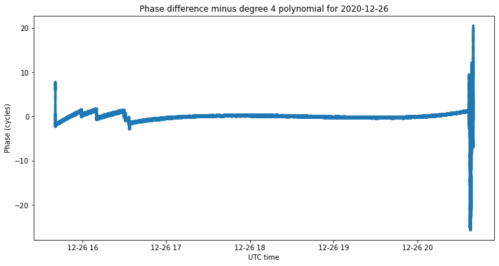
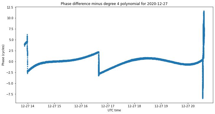
To assess the quality of the phase measurements, I compute the difference between 2h and 4g, fit a polynomial of degree 4 to the data, and plot the residual, as shown below. This shows cycle slips in the PLLs and any other problematic events, such as loss of lock at the end of the observation, when the spacecraft’s signal disappears. There are few cycle slips that can be fixed later by hand, so the PLL data is good enough to proceed.
The next step is phasing the observations. Since we do not have the precise right ascension and declination of the spacecraft, I take as phasing centre the dish pointing I used during each observation. This is right ascension 15.317 hours, declination -13.625 degrees for Saturday 26, and right ascension 15.34367 hours, declination -14.025 degrees for Sunday 27. The proper motion of the spacecraft was small enough that I could maintain the same dish pointing (in right ascension and declination coordinates) throughout each of the two observations.
For phasing, I use the 2h-4g baseline solution that I obtained with wideband interferometric observations of astronomical sources at different hour angles and declinations, using a centre frequency of 8475 MHz and a bandwidth of 30.72 MHz. This solution includes the ITRF coordinates of the baseline, an instrumental delay difference due to fibre optic cable runs of different lengths, etc, (this manifests itself as a phase slope versus frequency across the 30.72 MHz bandwidth), and an overall phase difference. To apply this solution to the narrowband carrier of Chang’e 5 at 8471.2 MHz, the delay is converted to its corresponding phase at the observation frequency, and applied together with the overall phase correction.
It is appropriate to remark that in both the observations of Chang’e 5 and the astronomical observations, the local oscillator of the telescope radio frequency conversion board was set to 8475 MHz, and the USRPs N32x were set to the same IF of 512 MHz. The USRPs used the same sample rate of 30.72 Msps in both cases also. The conversion of 8471.2 MHz down to baseband in the case of the recordings of Chang’e 5 is done in a GNU Radio flowgraph. The goal was to have the settings as similar as possible for the two very different kinds of signals, in order to avoid additional instrumental effects from appearing due to different settings.
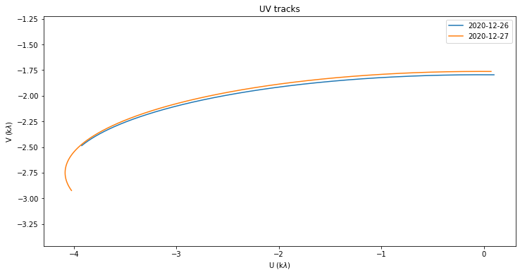
The figure below shows the UV coverage in each of the two observations. The tracks are very similar. The track for Saturday 26 is a bit shorter, because of the later start. The coverage in U is great, as it ranges between -4 and 0 kλ (the length of the baseline is near 5kλ). On the other hand, the coverage in V is not so good, since specially on the Saturday 26 it only sweeps approximately 0.5 kλ due to the late start.
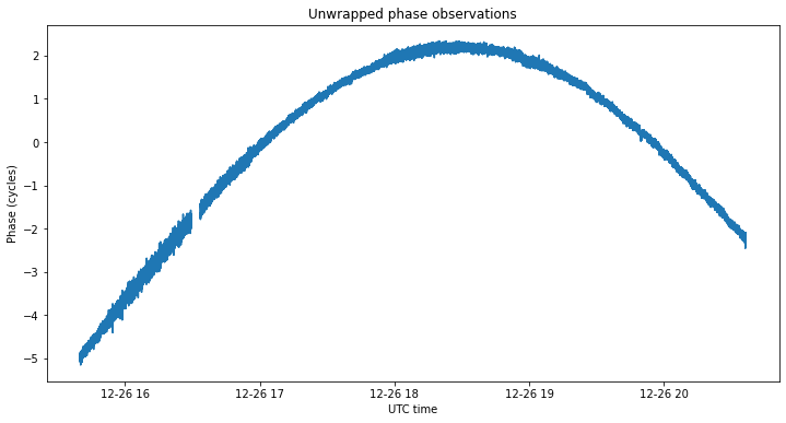
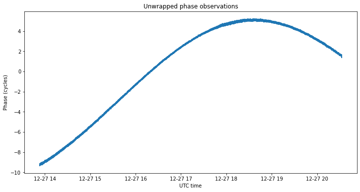
After phasing the observations, correcting the few cycle slips by hand, and flagging out some bad data, we obtain the figures below, which show the unwrapped visibility phases.
According to the Van Cittert-Zernike theorem, the visibility function for a source that is a Dirac delta at the coordinates \((l_0, m_0)\) in the image plane is\[V(u,v) = \exp(2\pi i (l_0 u + m_0 v)).\]Here the \((l,m)\) image plane coordinates indicate the offset in right ascension and declination from the phasing centre, measured in radians. The main idea to apply this theorem and solve for the source position using our unwrapped phase observations versus time \(\varphi(t)\) (measured in cycles) is to perform a linear least squares to solve\[l_0 u(t) + m_0 v(t) + C = \varphi(t).\]The integer \(C \in \mathbb{Z}\) is the phase ambiguity, which we also must solve for.
The problem in trying to apply this idea directly is that the spacecraft position in the image plane changes during the observation. Introducing a dependence of \(l_0\) and \(m_0\) on time \(t\) gives more unknowns than what the observation data can solve for, so it is important to model and correct the spacecraft movement in the image plane.
This movement is caused by two main contributions. The first is the spacecraft proper motion, which indicates how the spacecraft position in right ascension and declination coordinates changes. The second is diurnal parallax. Since the spacecraft was only at approximately 900000 km from Earth, its apparent position on the sky changes as the Earth rotates. In other words, the ATA-centric right ascension and declination coordinates of the spacecraft are different from the geocentric right ascension and declination coordinates.
These parameters are too much to solve with our interferometric data, so we lean on the orbit model that Bill Gray already has to model the spacecraft movement on the image plane. It is important to remark that we are only using Bill’s orbit for the relative movement on the image plane, not for the spacecraft’s absolute position, which is what we are going to solve for. Bill’s latest orbit solution and geocentric ephemerides can be found in this Chang’e 5 pseudo-MPEC.
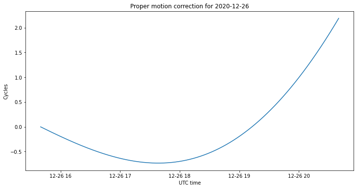
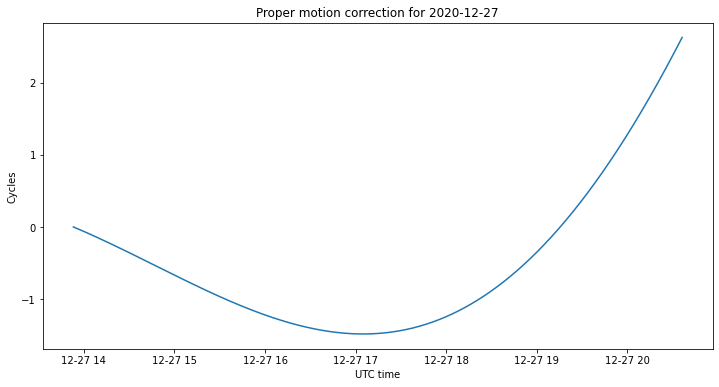
The spacecraft’s proper motion is almost given by a constant \(d\mathrm{RA}/dt\) and \(d\mathrm{DEC}/dt\) in each of the observations, since the right ascension and declination time derivatives change quite slowly. Nevertheless, I am using all the ephemerides from Bill’s orbit by computing for each epoch the difference in right ascension and declination with respect to the position at the start of the observation, so as to obtain the motion elapsed at that epoch. The phase change caused by proper motion is shown below. It only contributes to a couple of cycles throughout each observation.
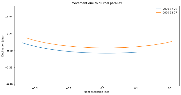
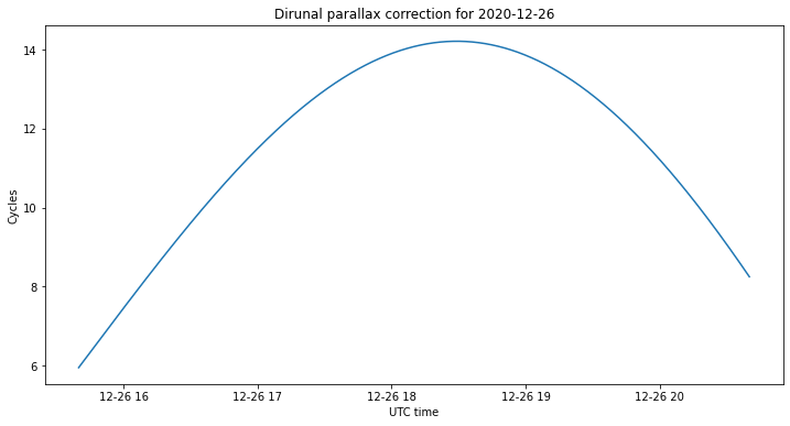
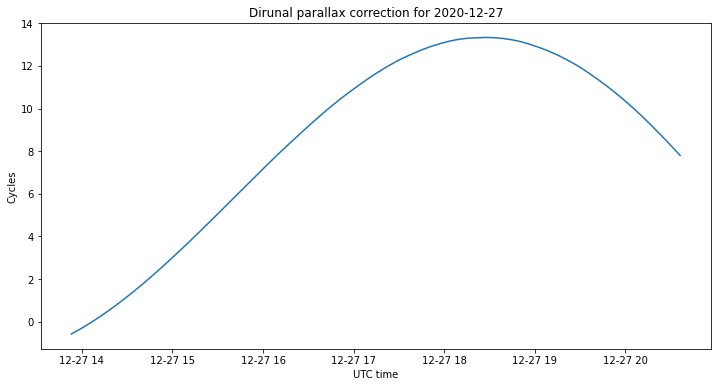
To model diurnal parallax as seen from ATA, I am using the right ascension, declination and distance coordinates from Bill’s ephemerides. I convert the geocentric right ascension and declination to ATA-centric right ascension and declination. Then I subtract from this the geocentric coordinates, in order to get only the displacement due to diurnal parallax. This is shown in the figure below. We see that the swing in right ascension is significant, as it’s as large as the dish beamwidth.
We convert this movement to phase cycles, obtaining the figures below. We see that the movement accounts for some 10 to 15 cycles, and closely resembles the unwrapped phase we got from our observations. In fact, most of the change in our phase observations is due to diurnal parallax.
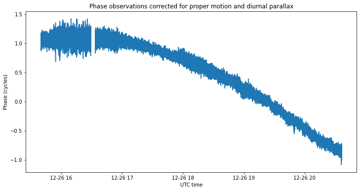
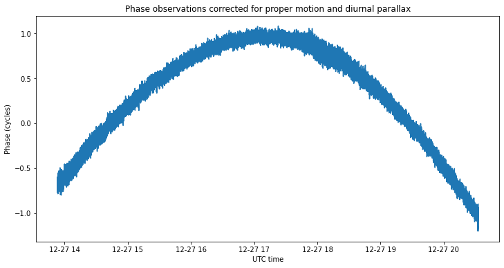
We now subtract the proper motion and diurnal parallax corrections from the observed data, and obtain the figures below. The change in phase throughout each observation is now only a couple of turns, which account for the object not being in the centre of the image plane.
With this phase data \(\varphi(t)\), now we perform a linear least squares to solve for \(l_0\), \(m_0\) and \(C\) in the equation\[l_0 u(t) + m_0 v(t) + C = \varphi(t).\]This solution is called a floating phase ambiguity fix, since we allow the phase ambiguity constant \(C\) to take any real value, rather than restricting it just to integer values. The values for \(l_0\) and \(m_0\) that we get are smaller than 0.2 degrees, so they are compatible with the error we expected in the dish pointing, which we took as the phasing centre of the image plane.
To obtain an integer phase ambiguity fix, we round the solution \(C\) to the nearest integer \(C_0 \in \mathbb{Z}\) and solve for \(l_0\) and \(m_0\) in\[l_0 u(t) + m_0 v(t) = \varphi(t) – C_0.\]Actually, by solving\[l_0 u(t) + m_0 v(t) = \varphi(t) – C_0 + k\]for small offsets \(k \in \mathbb{Z}\) we can assess whether the integer fix solution with \(C_0\) looks the only correct solution or if another integer fix might also be a good candidate.
The figure below shows the residuals for solutions obtained with small offsets and for the floating fix solution. The residuals have been averaged in windows of 100 seconds in order to reduce the noise so that the individual curves can be distinguished. We see that both the floating fix and the integer fix with an offset of zero look pretty good. The other integer fixes are worse and can be discarded.
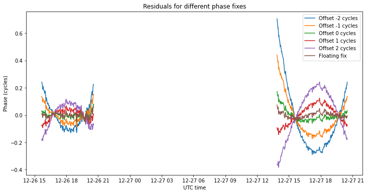
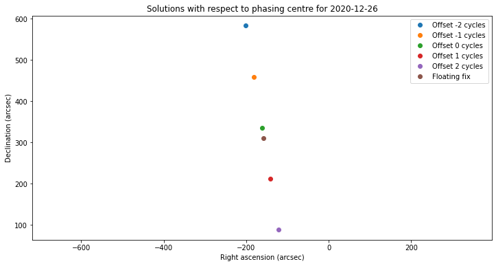
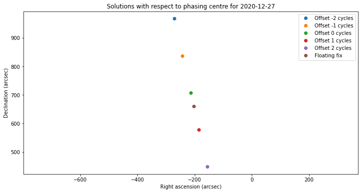
The positions of these solutions on the image plane are shown in the figure below. We see that they are quite closely spaced in right ascension, and not so much in declination, owing to the much better coverage in U.
Now the great question is whether to choose the integer fix (with zero cycles of offset) or the floating fix as the final solution. According to the Van Cittert-Zernike theorem, the integer fix is the correct one, but this requires the phase of the array to be calibrated correctly, because otherwise a constant non-integer error will show up in the phase observations. In my baseline solution I was able to obtain a phase calibration that worked correctly for the dozen of astronomical sources I observed. However, the phase measurements for Chang’e 5 are obtained in a different way, so I’m not completely confident that there isn’t an additional phase error showing up here.
The residuals for the floating and fixed solutions look quite similar and they are not completely flat, as it seems that there are still some unmodelled effects when correcting for the movement of Chang’e 5 on the image plane. Therefore, it is difficult to use the residuals to choose between the floating and fixed solutions.
In any case, the difference between the floating and integer solutions is on the order of 10 arcseconds of right ascension and 50 arcseconds of declination, so for me it seems reasonable to take the integer solution, and use this difference as our error bars.
The final solution becomes, thus, in geocentric right ascension and declination:
2020-12-26 15:39:56.159047 UTC - RA 15ʰ18ᵐ50.4206ˢ DEC -13°31′54.1711″
2020-12-27 13:53:02.170753 UTC - RA 15ʰ20ᵐ22.9492ˢ DEC -13°49′42.1772″
2 comments