On January 13, the SpaceX Transporter-3 mission launched many small satellites into a 540 km sun-synchronous orbit. Among these satellites were DELFI-PQ, a 3U PocketQube from TU Delft (Netherlands), which will serve for education and research, and EASAT-2 and HADES, two 1.5U PocketQubes from AMSAT-EA (Spain), which have FM repeaters for amateur radio. The three satellites were deployed close together with an Albapod deployer from Alba orbital.
While DELFI-PQ worked well, neither AMSAT-EA nor other amateur operators were able to receive signals from EASAT-2 or HADES during the first days after launch. Because of this, I decided to help AMSAT-EA and use some antennas from the Allen Telescope Array over the weekend to observe these satellites and try to find more information about their health status. I conducted an observation on Saturday 15 and another on Sunday 16, both during daytime passes. Fortunately, I was able to detect EASAT-2 and HADES in both observations. AMSAT-EA could decode some telemetry from EASAT-2 using the recordings of these observations, although the signals from HADES were too weak to be decoded. After my ATA observations, some amateur operators having sensitive stations have reported receiving weak signals from EASAT-2.
AMSAT-EA suspects that the antennas of their satellites haven’t been able to deploy, and this is what causes the signals to be much weaker than expected. However, it is not trivial to see what is exactly the status of the antennas and whether this is the only failure that has happened to the RF transmitter.
Readers are probably familiar with the concept of telemetry, which involves sensing several parameters on board the spacecraft and sending this data with a digital RF signal. A related concept is radiometry, where the physical properties of the RF signal, such as its power, frequency (including Doppler) and polarization, are directly used to measure parameters of the spacecraft. Here I will perform a radiometric analysis of the recordings I did with the ATA.