Experiments – Page 9 – Daniel Estévez

Planning Moon observations with my QO-100 station

There is a saying that goes like “even a broken clock is right twice a day”. In the same spirit, even a QO-100 station, which is installed with a fixed dish aiming to Es’hail 2, can sometimes be used for observing the Moon, as it happens to pass in front of the beam.

My station has a 1.2m offset dish with a GPSDO disciplined LNB. There are a few things that can be done when the Moon passes in front of the beam of the dish, such as measuring moon noise (though the increase in noise is only of around 10K with such a small dish), or receiving the 10GHz EME beacon or other EME stations. Therefore, it is interesting to know when these events happen, in order to prepare the observations.

I have made a simple Jupyter notebook that uses Astropy to compute the moments when the moon will pass through the beam of the dish (say, closer than 1º to the position of Es’hail 2 in the sky). Of course, the results are highly dependent on the location of the groundstation, so these are only valid for my groundstation and perhaps other groundstations in Madrid. Other people can run this notebook again using their data.

It turns out that each year the Moon passes roughly a dozen times in front of the dish beam. The next observation for me is on May 16. The separation in degrees between the centre of the Moon and the centre of the dish beam can be seen in the figure below.

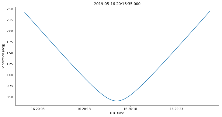
This notebook can be used to plan for transits of other astronomical objects, but besides the Moon and the Sun, there are no other objects that are visible at 10GHz with a small dish. It is well known when the Sun passes in front of the beam, since this disturbs communications with GEO satellites. This is called Sun outage and it happens during a few days around the equinoxes (a few weeks sooner or later, depending on the latitude of the station). On the other hand, the transits of the Moon happen throughout the whole year, at rather unpredictable moments, so I think this notebook is quite useful to plan observations.

Rain fade in the QO-100 downlink

The Amateur transponders of Es’hail 2 have their downlink in the 10GHz Amateur band. Even though the path to the satellite through the atmosphere is rather short, in extreme weather conditions it is possible to observe a small amount of fading in the signal. Two days ago there was intense rain over Madrid. As I’m often recording the power of the narrowband transponder beacons and the transponder noise floor, I have examined my data to see if the effect of the rain is visible.

The data is plotted in the figure below. See this post for an explanation of the measurements.

The power of the beacons is not very stable. It can vary up to 2 or 3dB along the course of the day. Therefore, it is not so easy to measure the drop in signal power caused by rain. However, it is noticeable that on April 24, between 05:00 and 17:00 UTC, the power of the beacons varies much more rapidly than usually. A small ripple of 0.5dB of amplitude is visible on the data. I think that this ripple is caused by varying rain intensity. Therefore, the data seems to suggest that the rains two days ago caused up to 0.5dB of fading in the signal.

As seen from my station, the satellite is at an elevation of \(\theta = 33.6^\circ\), so assuming a slant factor of \(1/\sin \theta = 1.8\), so taking a typical height of around 1km for the column of rain (see the corresponding METAR for Madrid airport), we get an attenuation on the order of 0.3dB/km. However, all the measurements used here are too imprecise to obtain any good conclusions. See this related post, in which I measured a 2.5dB increase in the noise floor at 12GHz during a hailstorm, but no change in signal power.

Diffraction in DSLWP-B lunar occultations

In February this year, the orientation of the orbit of DSLWP-B around the Moon was such that, when viewed from the Earth, it passed behind the Moon on every orbit. This opened up the possibility for recording the signal of DSLWP-B as it hid behind the Moon, thus blocking the line of sight path. The physical effect that can be observed in such events is that of diffraction. The power of the received signal doesn’t drop down to zero in a brick-wall fashion just after the line of sight is blocked, but rather behaves in an oscillatory fashion, forming the so called diffraction fringes.

The signal from DSLWP-B was observed and recorded at the Dwingeloo 25m radiotelescope for three days in February: 4th, 13th and 15th. During the first two days, an SSDV transmission was commanded several minutes before DSLWP-B hid behind the Moon, so as to guarantee a continuous signal at 436.4MHz to observe the variations in signal power as DSLWP-B went behind the Moon. On the 15th, the occultation was especially brief, lasting only 28 minutes. Thus, DSLWP-B was commanded to transmit continuously before hiding behind the Moon. This enabled us to also observe the end of the occultation, since DSLWP-B continued transmitting when it exited from behind the Moon. This is an analysis of the recordings made at Dwingeloo.

Detecting the Sprites from KickSat-2

The Sprites chipsats are tiny satellites built on a 3.5×3.5cm PCB with the bare minimum electronics to do something useful: a CC430 microcontroller with integrated FSK transceiver, an IMU, and solar cells.

The Sprites have been developed as part of the KickSat project, led by Zac Manchester, from Stanford University. The idea is to carry up to 128 Sprites in a cubesat and deploy them in a swarm once the cubesat is in orbit. The first test of this concept was done by the KickSat 3U cubesat in 2014. The test was a failure, since the Sprites couldn’t be deployed before KickSat reentered.

The second test was made this year with the KickSat-2 3U cubesat, a reflight of the KickSat mission carrying 104 Sprites. KickSat-2 was launched to the ISS onboard Cygnus NG-10 in November 2018 and deployed into orbit in February 2019.

On March 19, the Sprites were successfully deployed from KickSat-2, as Zac announced in Twitter, requesting help from the Amateur radio community to receive the signals from the Sprites at 437.240MHz. On March 22, Cees Bassa and Tammo Jan Dijkema tried to detect the Sprites by doing a planar scan with the Dwingeloo 25m radiotelescope. They were successful, detecting several transmissions from the Sprites in the waterfall. At that moment, the Sprites were up to 5 minutes ahead KickSat-2, due to their much higher drag to mass ratio. They all probably reentered a few days after this.

All the Sprites transmit in the same frequency using CDMA, so further analysis is required to identify which Sprites were observed by Dwingeloo. Zac said he was working on decoding the recording, however, I haven’t seen any results published yet. Here I show my analysis of the recording made at Dwingeloo. I manage to detect 4 different Sprites.

Measuring QO-100 beacons frequency

Continuing with my frequency measurements of Es’hail 2, I have now been measuring the frequency of the beacons of the QO-100 narrowband transponder for several days. The main goal of these frequency measurements is to use Doppler to study the orbit of Es’hail 2. Previously, I had been doing frequency measurements on the engineering beacons at 10706MHz and 11205MHz. However, these beacons are currently being transmitted on a MENA beam, so I’m quite lucky to be in Spain, as they can’t be received in many other parts of Europe.

During the in-orbit tests of Es’hail 2, the engineering beacons were transmitted on a global beam, and I performed some differential Doppler studies with Jean Marc Momple 3B8DU, in Mauritius. The engineering beacons are no longer any good for these kind of studies, since their area of coverage is small. Thus, I have started to measure the beacons in the narrowband transponder, which covers all the satellite footprint.

Recovering an image transmitted by DSLWP-B

The image accompanying this post has a nice story to it. It was taken by the Amateur camera in DSLWP-B, the Chinese microsatellite in lunar orbit. On February 27, a download of this image was attempted by transmitting the image in SSDV format in the 70cm band and receiving it in the Dwingeloo radiotelescope, in the Netherlands.

The download was attempted twice, but due to errors in the transmission, a small piece of the image was still missing. Today, the Amateur payload of DSLWP-B was active again, and the plan was to download the missing piece, as well as other images. However, after the payload turned on and transmitted its first telemetry beacons, we discovered that the image had been overwritten.

The camera on-board DSLWP-B has a buffer that stores the last 16 images taken. Any of these images can be selected to be transmitted (completely or partially) while the Amateur payload is active. An image can be taken manually by issuing a command from ground. Besides this, every time the Amateur payload powers on, an image is taken. Of course, taking new images overwrites the older ones.

This is what happened today. The image we wanted to download was the oldest one in the buffer and got overwritten as soon as the payload turned on. This is a pity, especially because there was another activation of the payload last Friday, but a large storm in Germany prevented Reinhard Kuehn DK5LA’ from moving his antennas safely, so the satellite couldn’t be commanded to start the download.

After seeing that the image had been overwritten, Tammo Jan Dijkema suggested that I try to recover manually the missing chunk in the recording made on February 27. As you can see, I was successful. This is a report of how I proceeded.

Changes to the QO-100 NB transponder settings

Yesterday, AMSAT-DL announced that the narrowband transponder of QO-100 was under maintenance and that some changes to its settings would be made. This was also announced by the messages of the 400baud BPSK beacon. Not much information was given at first, but then they mentioned that the transponder gain was reduced by 6dB and a few hours later the beacon power was increased by 5dB.

Since I am currently doing continuous power measurements of the transponder noise and the beacons, when I arrived home I could examine the changes and determine using my measurements that the transponder gain was reduced by 5dB (not 6dB) at around 15:30 UTC, and then the uplink power of the beacons was increased by 5dB at around 21:00 UTC, thus bringing the beacons to the same downlink power as before. In what follows, I do a detailed analysis of my measurements.

Es’hail 2 frequency measurements

After being busy with other projects, I have resumed my frequency measurements of the Es’hail 2 beacons. The last measurement I performed was made when the satellite reached its operational slot at 26ºE. After manoeuvering to this spot, the Doppler was very small, on the order of 0.8ppb peak-to-peak, indicating a very accurate geostationary orbit. Now Es’hail 2 has been two months in its operational slot, inaugurating its Amateur transponders on February 14 and entering commercial service on March 7.

I am curious about studying again the Doppler at this point in the mission, to see how accurate the GEO orbit is. I am also interested in collaborating with other Amateurs to perform differential Doppler measurements, as I did with Jean Marc Momple 3B8DU. Here I detail the first results of my measurements.

QO-100 beacons power

In the QO-100 (Es’hail 2) narrow band transponder, the recommendation for the adjustment of your downlink signal power is not to be stronger than the beacon. This was also the recommended usage of the old AO-40. Since the transponder has two beacons marking the transponder edges: a CW beacon marking the lower edge and a 400baud BPSK beacon marking the upper edge, there has been some debate on Twitter about which beacon does this recommendation refer to and what does “stronger” mean.

Of course, more formally, signal strength means power, which is a well defined physical concept, so there should be no argument about what does power mean. However, there are two different power measurements used for RF: average power and peak envelope power. I will assume that the recommendation refers to average power, not to peak envelope power. This makes more sense from the point of view of the power budget of the satellite amplifier (The total average power it needs to deliver is just the sum of the average powers of the signals of all the users, while the behaviour of the peak envelope power is much more complicated).

Also, I think that using peak envelope power for this restriction would be a very strict requirement on high PAPR signals. Note that the PAPR of CW is 0dB and the PAPR of BPSK is between 2 and 3dB, depending on the pulse shaping, so these are rather low PAPRs. For comparison, a moderately compressed SSB voice signal has a PAPR of 6dB.

In my opinion, the main problem with these discussions about “signal strength” is that many people are trying to judge power by looking at their waterfall or spectrum display and seeing what signal looks “higher”. This kind of measurement is not any good, because it doesn’t take signal bandwidth into account, depends on the FFT size, the window function, etc. It doesn’t help that many popular SDR software don’t have a good signal meter displaying the average power of the signal tuned in the passband.

In any case, I was curious about whether the power of the two beacons is the same and whether there is any interesting change over time. I have made a GNU Radio flowgraph that measures the power of each of the two beacons and of the transponder noise, and saves them to a file for later analysis.

Es’hail 2 stationed in 26ºE

If you’ve been following my posts about Es’hail 2, you’ll know that shortly after launch Es’hail 2 was stationed in a test slot at 24ºE. It remained in this slot until December 29, when it started to move to its operational slot at 26ºE. As of January 2, Es’hail is now stationed at 26ºE (25.8ºE, according to the TLEs).

The new GEO orbit at 26ºE is much more perfect than the orbit it had at 24ºE. This is to be expected for an operational orbit. Since December 30, I’ve been recording Doppler data of the satellite moving to its operational slot, and I have found some interesting effects of orbital dynamics in the data. This post is an account of these.