Since I published my Es’hail 2 Doppler measurement experiments, Jean Marc Momple 3B8DU has become interested in performing the same kind of measurements. The good thing about having several stations measuring Doppler simultaneously is that you can perform differential measurements, by subtracting the measurements done at each station. This eliminates all errors due to transmitter drift, since the drift is the same at both stations.
Of course, differential measurements need to be done with distant stations, to ensure different geometry that produces different Doppler curves in each station. Otherwise, the two stations see very similar Doppler curves, and subtracting yields nothing.
The good thing is that Jean Marc is in Mauritius, which, if you look at the map, is on the other side of the satellite compared to my station. The satellite is at 0ºN, 24ºE, my station is at 41ºN, 4ºW, and Jean Marc’s is at 20ºS, 58ºE. This provides a very good geometry for differential measurements.
Some days ago, Jean Marc sent me the measurements he had done on December 22, 23 and 24. This post contains an analysis of these measurements and the measurements I took over the same period, as well as some geometric analysis of Doppler.
It would be interesting if other people in different geographic locations join us and also perform measurements. As I’ll explain below, a station in Eastern Europe or South Africa would complement the measurements done from Spain and Mauritius well. If you want to join the fun, note a couple of things first: The Doppler is very small, around 1ppb (or 10Hz). Therefore, you need to have everything locked to a GPS reference, not only your LNB. Also, the change in Doppler is very slow. The Doppler looks like a sinusoidal curve with a period of one day. To obtain meaningful results, continuous measurements need to be done over a long period. At least 12 hours, and preferably a couple days.
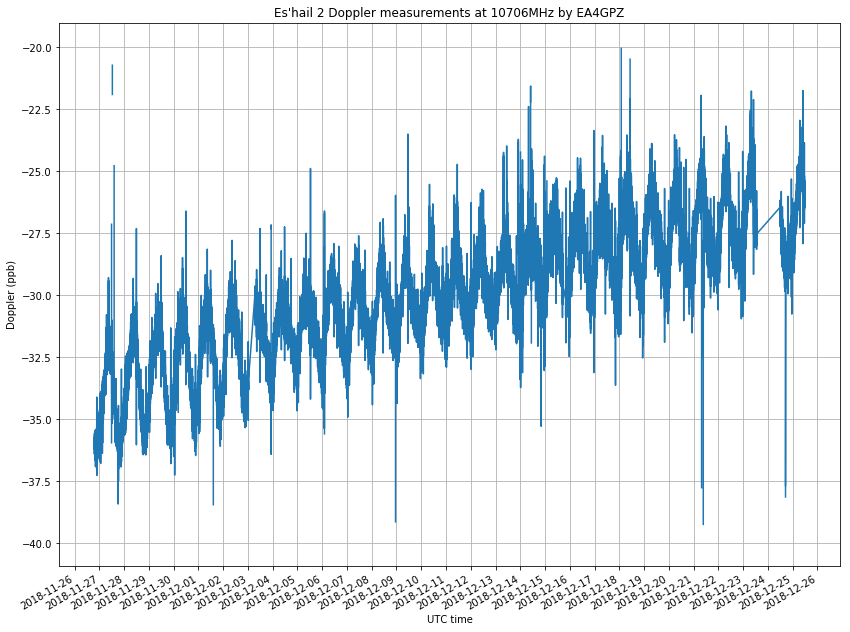
In a previous post I talked about my Doppler measurements of the Es’hail 2 10706MHz beacon. I’ve now been measuring the Doppler for almost a month and this is a follow-up post with the results. This experiment is a continuation of the previous post, so the measurement setup is as described there.
It is worthy to note that, besides the usual satellite movement in its geostationary orbit, which causes the small Doppler seen here, and the station-keeping manoeuvres done sometimes, another interesting thing has happened during the measurement period.
On 2018-12-13 at 8:00 UTC, the antenna where the 10706MHz beacon is transmitted was changed. Before this, it was transmitted on a RHCP beam with global coverage. After the change, the signal was vertically polarized and the coverage was regional. Getting a good coverage map of this beam is tricky, but according to reports I have received from several stations, the signal was as strong as usual in Spain, the UK and some parts of Italy, but very weak or inexistent in Central Europe, Brazil and Mauritius. It is suspected that the beam used was designed to cover the MENA (Middle East and North Africa) region, and that Spain and the UK fell on a sidelobe of the radiation pattern.
At some point on 2018-12-19, the beacon was back on the RCHP global beam, and it has remained like this until now.
The figure below shows my raw Doppler measurements, in parts-per-billion offset from the nominal 10706MHz frequency. The rest of the post is devoted to the analysis of these measurements.
Es’hail 2, the first geostationary satellite carrying an Amateur radio payload, was launched on November 15. I wrote a post studying the launch and geostationary transfer orbit, and I expected to track Es’hail 2’s manoeuvres by following the NORAD TLEs. However, for reasons not completely known, no NORAD TLEs were published during the first two weeks after launch.
On November 23, people found Es’hail 2 around the 24ºE geostationary orbital slot by receiving its Ku-band beacons at 10706MHz and 11205MHz. On November 27, NORAD TLEs started being published, confirming the position of Es’hail 2 around 24ºE. Since then, it has remained in this slot. Apparently, this is the slot that will be used for in-orbit test before moving the satellite to its operational slot on 25.5ºE or 26ºE.
Since November 27, I have been monitoring the frequency of the 10706MHz beacon to measure the Doppler. A geostationary satellite is never in a fixed location as seen from the Earth. It moves slightly due to imperfections in its orbit and orbital perturbations. This movement is detectable as a small amount of Doppler. Here I study the measurements I’ve been doing.
However, so far the reflection has been detected by hand by looking at the recording waterfalls. We don’t have any statistics about how often it happens or which conditions favour it. I want to make some scripts to process all the Dwingeloo recordings in batch and try to extract some useful conclusions from the data.
Here I show my first script, which computes the power of the direct and reflected signals (if any). The analysis of the results will be done in a future post.
In my last post, I detailed the DSLWP-B camera planning for the beginning of November. There, I used orbital state taken from the 20181027 tracking file to compute good times to take images of the Moon and the Earth, especially looking for an Earthrise-like image.
Now that the planned dates are closer, it is good to rerun the calculations with a newer orbital state. It turns out that there has been an important change in the mean anomaly, which shifts all the predictions by a few hours.
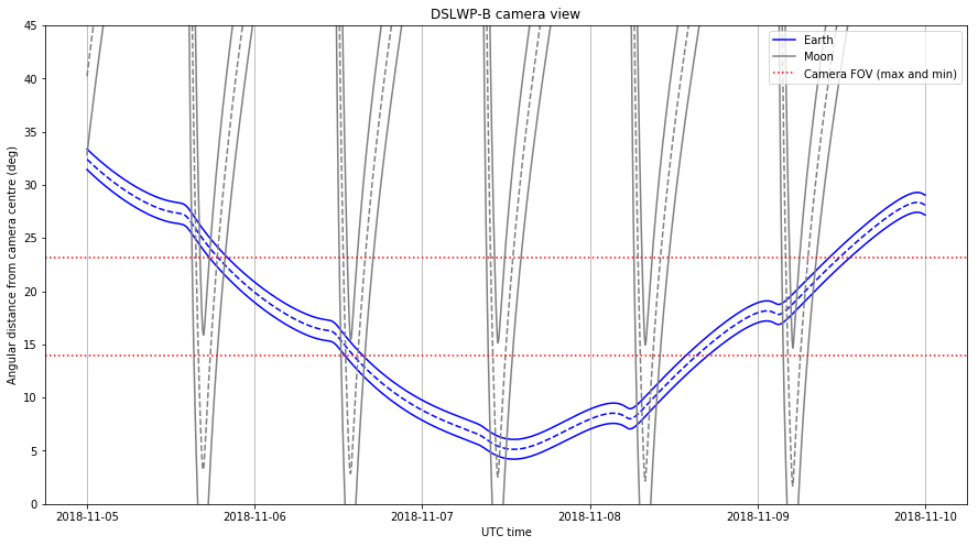
I have spoken in other occasions about planning the appropriate times to take pictures with the DSLWP-B Inory eye camera. In the beginning of October there was a window that allowed us to take images of the Moon and Earth. A lunar month after this we have new Moon again, so it is an appropriate time to take images with the camera.
This time, the Moon will pass nearer to the centre of the image than on October, and at certain times the Earth will hide behind the Moon, as seen from the camera. This opens up the possibility for taking Earthrise pictures such as the famous image taken during the Apollo 8 mission.
I have updated my camera planning Jupyter notebook to compute the appropriate moments to take images. The image below shows my usual camera field of view diagram.
The vertical axis represents the angular distance in degrees between each object and the centre of the image (Assuming the camera is pointing perfectly away from the Sun. In real life we can have a couple degrees of offset). The red lines represent the limits of the camera field of view, which are measured between the centre and the nearest edge, and between the centre and one corner. Everything between these two lines will only appear if the camera rotation is adequate. Everything below the lower line is guaranteed to appear, regardless of rotation.
We see that between November 6th and November 9th there are four times when the camera will be able to image the Earth and the Moon simultaneously. On the 6th it is almost guaranteed that the Earth will appear inside the image, and on the 9th it depends on the orientation of the camera. On the 7th and 8th it is guaranteed that the Earth will be in the image.
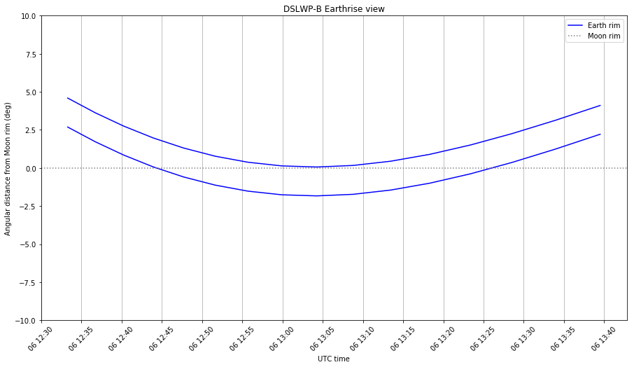
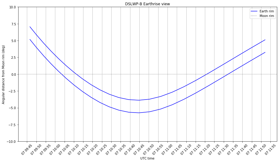
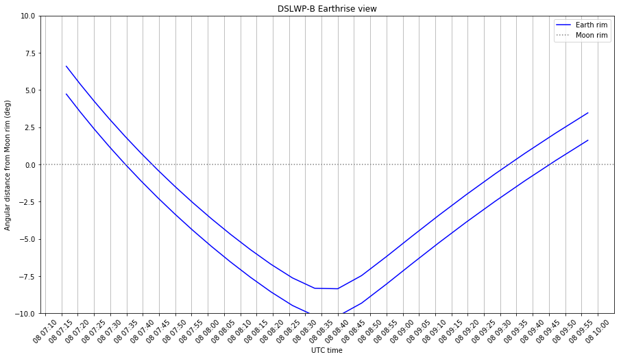
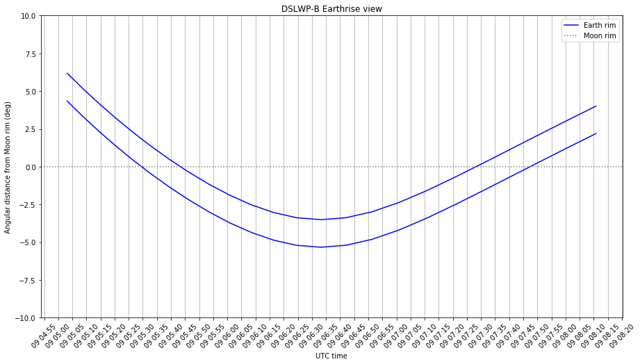
To compute appropriate times for taking an Earthrise picture, I have made the graph below. This shows the angular distance between the Earth and the rim of the Moon. If the distance is negative, the Earth is hidden by the Moon. We see that the Earth hides behind the lunar disc on each of the four days mentioned above.
In the figures below, we zoom in each of the events. In this level of zoom we can plot the “inner” and “outer” Earth rim, so we can see when the Earth is partially hidden by the Moon.
On November 6th the situation is the most interesting in my opinion. It turns out the the Earth will not even hide completely between the Moon. In theory, a tiny sliver will remain visible. Also, it will take more time for the Earth to hide behind the Moon and then reappear. As we will see, the next days this will happen faster. Here, it takes 15 minutes for the Earth to hide, and another 15 minutes to reappear. It spends 10 minutes almost hidden.
It can be a good idea to take a series of 10 images with an interval of 5 minutes between each image, and spanning from 12:40 UTC to 13:30 UTC, to get a good coverage for this event.
On November 7th the Earth goes deeper into the lunar disc, taking 5 minutes to hide, spending 70 minutes hidden, and taking 10 minutes to reappear.
On November 8th the Earth goes even deeper into the lunar disc. It takes around 7 minutes to hide, spends 105 minutes hidden and takes 10 minutes to reappear.
On November 9th the configuration is quite similar to November 7th, but the hiding speed is slower. It takes 15 minutes to hide, spends 100 minutes hidden and takes 15 minutes to reappear.
Overall, I think that the best would be to take a good series of images on November 6th, since this shallow occultation is a rarer event. The challenge will be perhaps to download all the images taken during these days. On average, I think we are downloading around 2 new images per 2 hour activation, taking into account repeats due to lost blocks and dead times. DSLWP-B is able to store 16 images onboard, and every time the UHF transmitter comes on, a new image is taken, overwriting an old image (more information in this post). Thus, if we take many images during these days, we have the danger of overwriting some when trying to download them over the next few days.
Perhaps a good strategy is to arrange for a series of 10 images to be taken on the 6th, and then programming the UHF transmitter to take an image as the Earth comes out of its occultation on the 7th, 8th and 9th. In this way, the 2 hour periods of these three days can be used to download some of the images taken on the 6th, and there are still 3 images of margin in the buffer in case something goes wrong during the downloads over the next few days.
In my previous post I showed that during the DSLWP-B observation on 2018-10-27 17:20 UTC, the orbit of DSLWP-B would take it behind the Moon. This doesn’t happen every orbit (read as every day, since the orbit period is around 22 hours). It depends on the angle from which the orbit is viewed from Earth, and hence on the lunar phase.
Knowing beforehand when DSLWP-B will hide behind the Moon allows to perform radio occultation studies. These consist in measuring the RF signal from DSLWP-B as it gets blocked by the lunar disc. Interesting phenomena such as diffraction can be observed.
I have calculated the occultations that will be visible from the Dwingeloo radiotelescope in the remaining part of this year.
I have already spoken about the Moonbounce signal from DSLWP-B in several posts. To sum up, DSLWP-B is a Chinese satellite that is orbiting the Moon since May 25. The satellite has an Amateur payload that transmits GMSK and JT4G telemetry in the 70cm Amateur satellite band. This signal can be received by well equipped groundstations on Earth, including the 25m radiotelescope at Dwingeloo, in the Netherlands (and also by much smaller stations).
The people at Dwingeloo publish the recordings that they make of the RF signal. In two of these recordings, the signal from DSLWP-B is received not only via the direct path, but also through a reflection off the Moon’s surface. The reflected signal is around 25dB weaker, usually has a different Doppler shift, and has a Doppler spread of around 50 to 200Hz.
What I find most interesting about this is that of all the days that Dwingeloo has observed DSLWP-B, in only two of them (on 2018-10-07 and 2018-10-19) the Moonbounce signal has been visible. Mathematically, using a specular reflection on a sphere model, whenever the satellite is visible directly, there is also a ray from the spacecraft that reflects off the lunar surface and arrives at the groundstation (see the proof here). Therefore, I think that there must be something about the particular geometry of the days 7th and 19th that made the Moon reflections relatively stronger and hence detectable. Here I use GMAT to study the orbital geometry when the reflections were received.
On the other hand, JT4G is a digital mode designed for Earth-Moon-Earth microwave communications, so it is tolerant to high Doppler spreads. However, the reflections of the B0 transmitter at 435.4MHz, which contained the JT4G transmissions, were very weak, so I had not attempted to decode the JT4G Moonbounce signal.
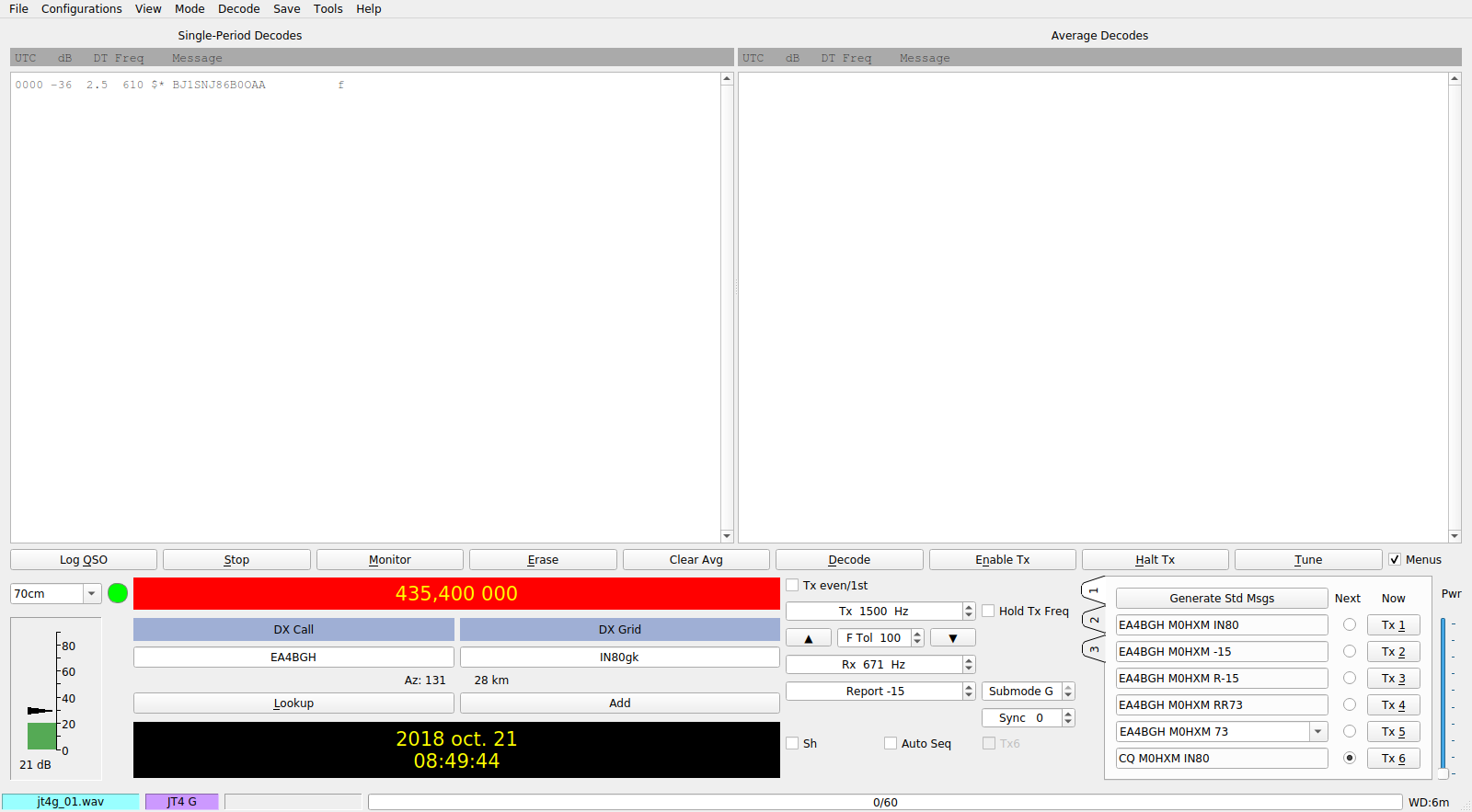
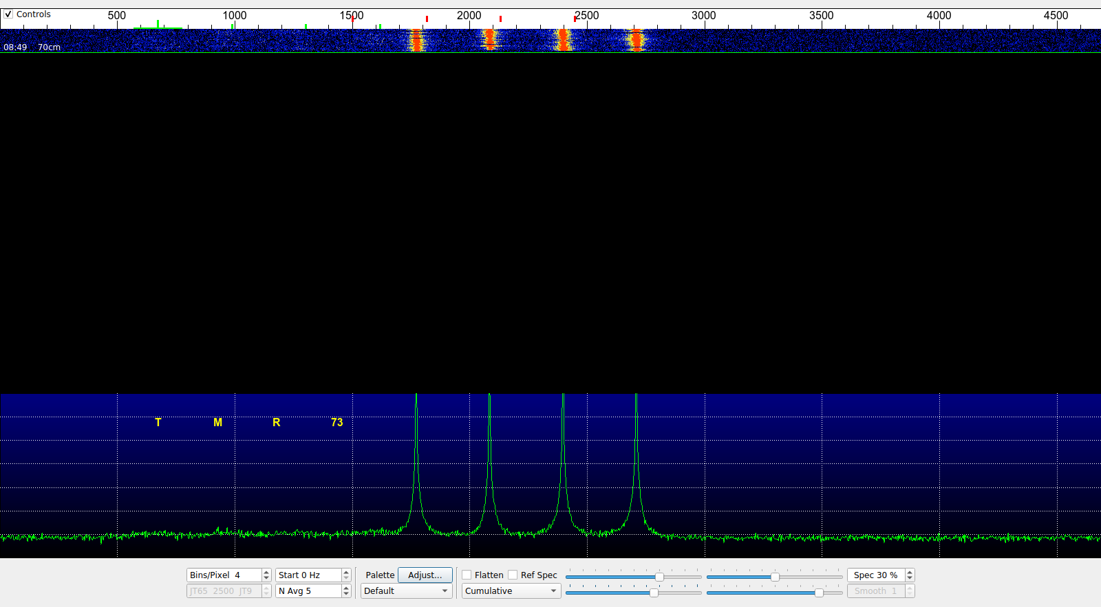
On 2018-10-19, the Moonbounce signal from DSLWP-B was again visible in Dwingeloo’s recordings. I have used the 2018-10-19T17:53:35 435.4MHz recording and managed to decode the Moonbounce signal of one out of the five JT4G transmissions that appear in the recording.
To extract the data from the recording to WAV files that can be read by WSJT-X, I have used the following Jupyter notebook. Then I have used WSJT-X version 2.0.0-rc3 to try to decode the Moonbounce signal. Since the JT4 decoder only decodes a single signal at the selected frequency, it is enough to select the frequency of the Moonbounce signal in WSJT-X. The direct signal will not be decoded, even though it is also present in the WAV file.
The only transmission that I have managed to decode was made at 18:11 UTC. The two screenshots below show WSJT-X decoding the WAV file extracted from the recording.
WSJT-X decoding the Moonbounce signal
Note the direct signal with a lowest tone at 1800Hz. The reflected signal is very faint, with a lowest tone at 700Hz. The Doppler spread of the reflected signal is large, approximately 200Hz, although it is difficult to judge from the spectrum.
When the WAV file is created, I also compensate for a linear frequency drift of 25Hz per minute due to Doppler, but this is not essential to obtain a valid decode.
WSJT-X decoding the Moonbounce signal
The WAV file that produces a decode can be downloaded here. This file can be opened directly by WSJT-X.
In one of my latest posts I commented on the Moonbounce signal of the Chinese lunar satellite DSLWP-B, as received in Dwingeloo. In the observation made in 2018-10-07 Cees Bassa discovered a signal in the waterfall of the Dwingeloo recordings that seemed to be a reflection off the Moon of DSLWP-B’s 70cm signal. My analysis showed that the Doppler of this signal was compatible with a specular reflection on the lunar surface.
In this post I study the cross-correlation of the Moonbounce signal against the direct signal. This gives some information about how the radio signals behave when reflecting off the Moon. Essentially, we compute the Doppler spread and time delay of the Moonbounce channel.