orbital dynamics – Page 5 – Daniel Estévez

DSLWP-B lunar impact prediction

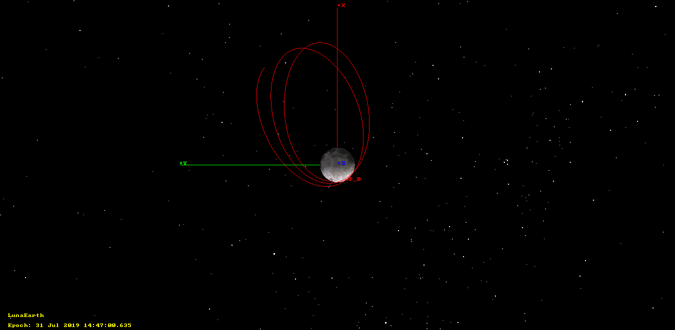
In my last post, I spoke about the future lunar impact of DSLWP-B on July 31. Edgar Kaiser DF2MZ asked over on Twitter if the impact would be visible from Earth. As I didn’t know the answer, I have made a simulation in GMAT to find this out.

The figure below shows the orbit of DSLWP-B between July 28 12:00 UTC and the moment of impact, on July 13 14:47 UTC. The orbital state used for DSLWP-B is the 20190426 tracking file from dslwp_dev. The reference frame is arranged so that the +X axis points towards the Earth, and the Y axis lies on the Earth-Moon orbital plane. As we can see, unfortunately, the impact will happen on the far side of the Moon, where it is not observable from Earth.

Future impact of DSLWP-B on the far side of the Moon

However, it is possible to arrange a manoeuvre to modify the orbit slightly and make the impact point fall on the near side of the Moon, where it is visible from Earth. In the previous post we observed that, ignoring the collision with the lunar surface, the periapsis radius would continue to decrease after July 31, until reaching a minimum value in January 2020.

Therefore, it is possible to raise the periapsis radius slightly in order to delay the collision approximately half a lunar month, so that the periapsis faces the Earth at the moment of impact. The delta-v required to make this manoeuvre is small, as the adjustment to the orbit is subtle.

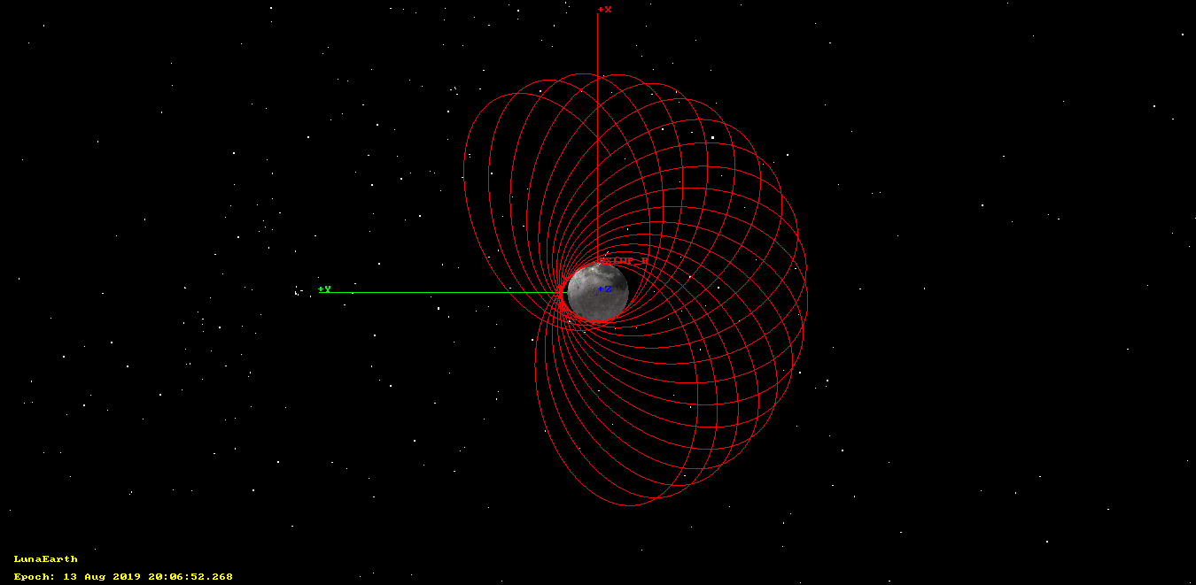
For instance, performing a prograde burn of 7m/s at the first apoapsis after July 1 delays the collision until August 13, producing an impact in the near side of the Moon. The resulting orbit can be seen in the figure below, which shows the path of DSLWP-B between July 28 and the moment of impact.

Impact of DSLWP-B on the near side of the Moon if a correction manoeuvre is applied

Adjusting the delta-v more precisely would make it possible even to control the time of the impact, so as to guarantee that the Moon will be in view of the groundstations at China and The Netherlands when the collision happens. However, this adjustment requires a very precise delta-v and is quite sensitive to the orbital state, so perhaps it is not feasible without performing a precise orbit determination and maybe some smaller correction manoeuvres following the periapsis raise.

Another possible problem that can affect the prediction of the impact point are the perturbations of the orbit caused by the lunar mascons, which can be noticeable when the altitude of the orbit starts getting small, and which haven’t been considered very carefully in this simulation (the non-spherical gravity of the Moon was only simulated up to degree and order 10).

The GMAT script used for this post can be found here.

DSLWP-B deorbit and mission end

On January 24, the periapsis of the lunar orbit of DSLWP-B was lowered approximately by 500km, so that orbital perturbations would eventually force the satellite to collide with the Moon. This was done to put an end to the mission and to avoid leaving debris in orbit. It is expected that the collision will happen at the end of July, so there are only three months left now for the DSLWP-B mission. Here I look at the details of the deorbit.

Es’hail 2 frequency measurements

After being busy with other projects, I have resumed my frequency measurements of the Es’hail 2 beacons. The last measurement I performed was made when the satellite reached its operational slot at 26ºE. After manoeuvering to this spot, the Doppler was very small, on the order of 0.8ppb peak-to-peak, indicating a very accurate geostationary orbit. Now Es’hail 2 has been two months in its operational slot, inaugurating its Amateur transponders on February 14 and entering commercial service on March 7.

I am curious about studying again the Doppler at this point in the mission, to see how accurate the GEO orbit is. I am also interested in collaborating with other Amateurs to perform differential Doppler measurements, as I did with Jean Marc Momple 3B8DU. Here I detail the first results of my measurements.

Es’hail 2 stationed in 26ºE

If you’ve been following my posts about Es’hail 2, you’ll know that shortly after launch Es’hail 2 was stationed in a test slot at 24ºE. It remained in this slot until December 29, when it started to move to its operational slot at 26ºE. As of January 2, Es’hail is now stationed at 26ºE (25.8ºE, according to the TLEs).

The new GEO orbit at 26ºE is much more perfect than the orbit it had at 24ºE. This is to be expected for an operational orbit. Since December 30, I’ve been recording Doppler data of the satellite moving to its operational slot, and I have found some interesting effects of orbital dynamics in the data. This post is an account of these.

An STRF crash course

Recently, the STRF satellite tracking toolkit for radio observations by Cees Bassa has been gaining some popularity. This toolkit allows one to process RF recordings to extract frequency measurements and perform TLE matching and optimization via Doppler curves. Unfortunately, there is not a lot of documentation for this toolkit. There are some people that want to use STRF but don’t have a clear idea of where to start.

While I have tested very briefly STRF in the past, I had never used it for doing any serious task, so I’m also a newcomer. I have decided to test this tool and learn to use it properly, writing some sort of walk-through as I learn the main functionality. Perhaps this crash course will be useful to other people that want to get started with STRF.

As I have said, I’m no expert on STRF, so there might be some mistakes or omissions in this tutorial that hopefully the experts of STRF will point out. The crash course is organized as a series of exercises that explain basic concepts and the workflow of the tools. The exercises revolve around an IQ recording that I made of the QB50 release from ISS in May 2017. That recording is interesting because it is a wide band recording of the full 70cm Amateur satellite band on an ISS pass on May 29. During a few days before this, a large number of small satellites had been released from the ISS. Therefore, this recording is representative of the TLE lottery situation that occurs after large launches, where the different satellites haven’t drifted much yet and one is trying to match each satellite to a TLE.

The IQ recording can be downloaded here. I suggest that you download it and follow the exercises on your machine. After you finish all the exercises, you can invent your own. Certainly, there is a lot that can be tried with that recording.

A number of supporting files are created during the exercises. For reference, I have created a gist with these files.

One month of Es’hail 2 Doppler data

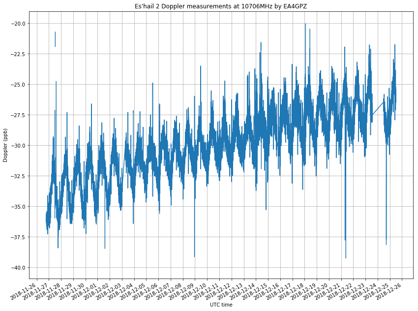
In a previous post I talked about my Doppler measurements of the Es’hail 2 10706MHz beacon. I’ve now been measuring the Doppler for almost a month and this is a follow-up post with the results. This experiment is a continuation of the previous post, so the measurement setup is as described there.

It is worthy to note that, besides the usual satellite movement in its geostationary orbit, which causes the small Doppler seen here, and the station-keeping manoeuvres done sometimes, another interesting thing has happened during the measurement period.

On 2018-12-13 at 8:00 UTC, the antenna where the 10706MHz beacon is transmitted was changed. Before this, it was transmitted on a RHCP beam with global coverage. After the change, the signal was vertically polarized and the coverage was regional. Getting a good coverage map of this beam is tricky, but according to reports I have received from several stations, the signal was as strong as usual in Spain, the UK and some parts of Italy, but very weak or inexistent in Central Europe, Brazil and Mauritius. It is suspected that the beam used was designed to cover the MENA (Middle East and North Africa) region, and that Spain and the UK fell on a sidelobe of the radiation pattern.

At some point on 2018-12-19, the beacon was back on the RCHP global beam, and it has remained like this until now.

The figure below shows my raw Doppler measurements, in parts-per-billion offset from the nominal 10706MHz frequency. The rest of the post is devoted to the analysis of these measurements.

Studying Es’hail 2 Doppler

Es’hail 2, the first geostationary satellite carrying an Amateur radio payload, was launched on November 15. I wrote a post studying the launch and geostationary transfer orbit, and I expected to track Es’hail 2’s manoeuvres by following the NORAD TLEs. However, for reasons not completely known, no NORAD TLEs were published during the first two weeks after launch.

On November 23, people found Es’hail 2 around the 24ºE geostationary orbital slot by receiving its Ku-band beacons at 10706MHz and 11205MHz. On November 27, NORAD TLEs started being published, confirming the position of Es’hail 2 around 24ºE. Since then, it has remained in this slot. Apparently, this is the slot that will be used for in-orbit test before moving the satellite to its operational slot on 25.5ºE or 26ºE.

Since November 27, I have been monitoring the frequency of the 10706MHz beacon to measure the Doppler. A geostationary satellite is never in a fixed location as seen from the Earth. It moves slightly due to imperfections in its orbit and orbital perturbations. This movement is detectable as a small amount of Doppler. Here I study the measurements I’ve been doing.

Es’hail 2 launch in GMAT

After a long wait by many Amateur radio operators, Es’hail 2, the first geostationary satellite carrying an Amateur radio transponder launched yesterday on a SpaceX Falcon 9 Full Thrust from the historical LC-39A pad in Kennedy Space Centre, which was used by many Apollo and Space Shuttle launches in the past.

Es’hail 2 is the second communications satellite operated by the Qatari company Es’hailSat. It was built by Mitsubishi Electric Corporation (MELCO). It carries several Ku and Ka band transponders intended for digital television, Internet access and other data services. It also carries an Amateur radio payload designed by AMSAT-DL, in collaboration with the Qatar Amateur Radio Society. The payload has two transponders, with S-band uplink and X-band downlink. One of the transponders is 250kHz wide and intended for narrowband modes, and the other one is 8MHz wide and intended for DVB-S and other wideband data modes.

SpaceX live-streamed the launch, and the recording can be seen in YouTube. Today, Space-Track has published the first TLEs for Es’hail 2 and the second stage of the Falcon 9 rocket. Here I look at these TLEs using GMAT.

Geometry for DSLWP-B Moonbounce

I have already spoken about the Moonbounce signal from DSLWP-B in several posts. To sum up, DSLWP-B is a Chinese satellite that is orbiting the Moon since May 25. The satellite has an Amateur payload that transmits GMSK and JT4G telemetry in the 70cm Amateur satellite band. This signal can be received by well equipped groundstations on Earth, including the 25m radiotelescope at Dwingeloo, in the Netherlands (and also by much smaller stations).

The people at Dwingeloo publish the recordings that they make of the RF signal. In two of these recordings, the signal from DSLWP-B is received not only via the direct path, but also through a reflection off the Moon’s surface. The reflected signal is around 25dB weaker, usually has a different Doppler shift, and has a Doppler spread of around 50 to 200Hz.

What I find most interesting about this is that of all the days that Dwingeloo has observed DSLWP-B, in only two of them (on 2018-10-07 and 2018-10-19) the Moonbounce signal has been visible. Mathematically, using a specular reflection on a sphere model, whenever the satellite is visible directly, there is also a ray from the spacecraft that reflects off the lunar surface and arrives at the groundstation (see the proof here). Therefore, I think that there must be something about the particular geometry of the days 7th and 19th that made the Moon reflections relatively stronger and hence detectable. Here I use GMAT to study the orbital geometry when the reflections were received.

DSLWP-B Moonbounce

If you have been following my latest posts, you will know that a series of observations with the DSLWP-B Inory eye camera have been scheduled over the last few days to try to take and download images of the Moon and Earth (see my last post). In a future post I will do a chronicle of these observations.

On October 6 an image of the Moon was taken to calibrate the exposure of the camera. This image was downlinked on the UTC morning of October 7. The download was commanded by Reinhard Kuehn DK5LA and received by the Dwingeloo radiotelescope.

Cees Bassa observed that in the waterfalls of the recordings made in Dwingeloo a weak Doppler-shifted signal of the DSLWP-B GMSK signal could be seen. This signal was a reflection off the Moon.

As far as I know, this is the first reported case of satellite-Moon-Earth (or SME) propagation, at least in Amateur radio. Here I do a Doppler analysis confirming that the signal is indeed reflected on the Moon surface and do some general remarks about the possibility of receiving the SME signal from DSLWP-B. Further analysis will be done in future posts.