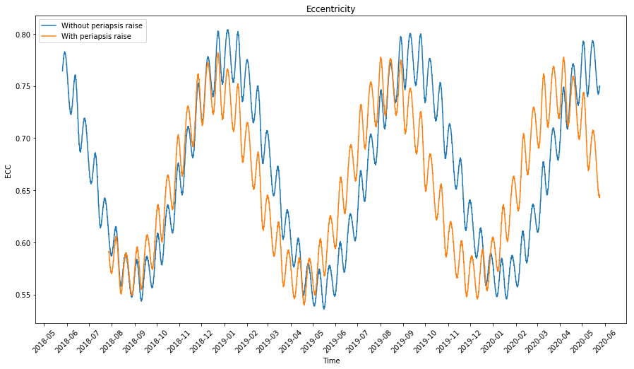
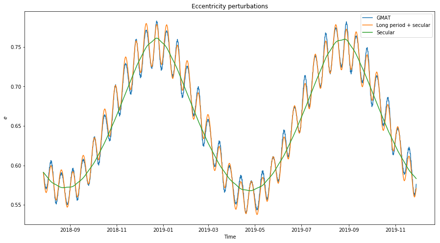
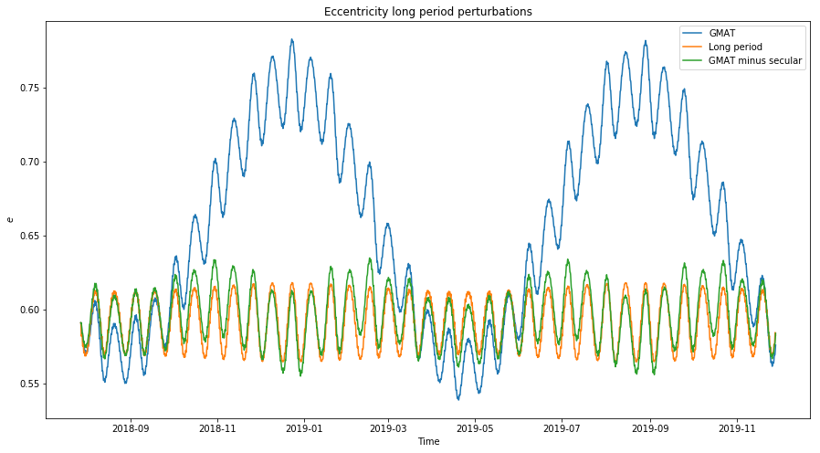
Ever since simulating DSLWP-B’s long term orbit with GMAT, I wanted to understand the cause of the periodic perturbations that occur in some Keplerian elements such as the eccentricity. As a reminder from that post, the eccentricity of DSLWP-B’s orbit shows two periodic perturbations (see the figure below). One of them has a period of half a sidereal lunar month, so it should be possible to explain this effect from the rotation of the Moon around the Earth. The other has a period on the order of 8 or 9 months, so explaining this could be more difficult.
In this post I look at how to model the perturbations of the orbit of a satellite in lunar orbit, explaining the behaviour of the long term orbit of DSLWP-B.
The Wikipedia contains a good introduction to the theory of perturbations of the Keplerian elements. The main idea is that if the function \(g = g(x_1,x_2,x_3,v_1,v_2,v_3)\) is a constant of motion for a Keplerian orbit and \((h_1,h_2,h_3)\) is a perturbing force per unit mass, then\[\dot{g} = \frac{\partial g}{\partial v_1} h_1 + \frac{\partial g}{\partial v_2} h_2 + \frac{\partial g}{\partial v_2} h_2.\] Usually, we study \(\Delta g\), the change in \(g\) over an orbit revolution. This is computed by integrating \(\dot{g}\) over a revolution and assuming that the perturbed orbit is very close to the Keplerian orbit, so the trajectory of the orbit can be taken to be the Keplerian orbit. Thus,\[\Delta g = \int_0^{2\pi} \dot{g} \frac{r^2}{\sqrt{\mu p}}\, d\theta,\]where \(\theta\) is the true anomaly, \(p = a(1-e^2)\) is the semi-latus rectum, \(r\) is the orbit radius, and \(\mu = GM\) is the gravitational parameter (here \(a\) is the semi-major axis, \(e\) the eccentricity, \(G\) the universal gravitational constant, and \(M\) the mass of the central body).
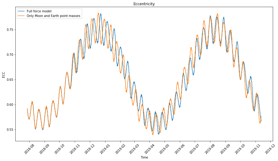
By doing some simulations with GMAT, I quickly determined that the major contributor to the perturbations of the orbit of DSLWP-B was Earth’s gravity. Below you can see two simulations in GMAT for the eccentricity. One of them uses the complete force model with lunar spherical harmonics, point masses for the Earth, Sun and planets, solar radiation, and relativistic effects, and the other one only uses the point mass forces for the Moon and Earth. The result is so similar that we can restrict ourselves to the study of the Earth’s point mass gravity as the only perturbing force. Here, and in the rest of this post I am using the first line of the 20160727a tracking file in dslwp_dev as the state vector for DSLWP-B’s orbit.
The Wikipedia article contains a derivation of the perturbations of each of the Keplerian elements over one revolution, in terms of a general force per unit mass \(h = (h_1,h_2,h_3)\), and worked out examples for some particular forces (including the force due to the oblateness of the central body). To apply these ideas we first need to determine the force \(h\), which in our case is the gravitational force of the Earth.
My first approach was as follows (note that this is completely wrong; more on that later). We consider a reference system centred on the Moon and denote by \(r\) the position of our satellite and \(r_1\) the position of the Earth according to this system. Then the gravitational force per unit mass exerted by the Earth on the satellite is\[h = -\mu_1 \frac{r_1-r}{\|r_1-r\|^3},\]where \(\mu_1\) is Earth’s gravitational parameter. Since the satellite is in lunar orbit, we assume that \(\|r\| \ll \|r_1\|\) so we can approximate \(h\) as\[h \approx -\mu_1 \frac{r_1}{\|r_1\|^3}.\]
Since the orbital period is much smaller than a lunar month, we can assume that \(r_1\) is constant over each revolution. Therefore, the force \(h\) does not depend on time, and so \(\Delta g\) is a linear function of \(h\).
Basing my calculations on the Wikipedia article, I worked out the perturbations of each Keplerian element for a constant force \(h\), but I got stuck, since I couldn’t manage to match what I saw in my GMAT simulations. Indeed, since \(h\) has a period of one lunar month, the perturbations of the Keplerian elements will also have a period of one lunar month, not half a lunar month as the GMAT simulations show.
I couldn’t find the problem with my calculations, so I started reading the book Introduction to the Theory of Flight of Artificial Earth Satellites by P.E. El’Yasberg. This book is very well written and Chapter 16 is devoted to a study of the perturbations caused on Earth-orbiting satellites by the Moon and the Sun. Our situation about the perturbation of a lunar-orbiting satellite by the Earth is analogous and all the results in the book can be applied.
Reading this book I found that the problem with my reasoning explained above was a very basic conceptual error in physics. The force\[-\mu_1 \frac{r_1-r}{\|r_1-r\|^3}\] is written in a non-inertial frame of reference, and Newton’s laws can only be applied in inertial reference systems.
The correct force acting on the satellite should be calculated as follows. We write as \(r_0\) the position of the Moon on an inertial frame of reference centred on the Earth-Moon system barycentre. Then\[\ddot{r_0} = -\mu_1 \frac{r_1}{\|r_1\|^3}.\] If \(s = r + r_0\) is the position of the satellite in this inertial reference system, then\[\ddot{s} = -\mu_0 \frac{r}{\|r\|^3} – \mu_1\frac{r-r_1}{\|r-r_1\|^3},\]where \(\mu_0\) is the Moon’s gravitational parameter. Therefore\[\ddot{r} = -\mu_0 \frac{r}{\|r\|^3} – \mu_1\left(\frac{r-r_1}{\|r-r_1\|^3} – \frac{r_1}{\|r_1\|^3}\right).\]The left summand on the right hand side of this expression is the Keplerian force due to the Moon. The right summand is the correct expression for the perturbing force\[h = – \mu_1\left(\frac{r-r_1}{\|r-r_1\|^3} – \frac{r_1}{\|r_1\|^3}\right).\]
The book by El’Yasberg contains a first order approximation for the perturbing force\[h \approx \mu_1\frac{\|r\|}{\|r_1\|^3}\left(3\frac{\langle r, r_1\rangle}{\|r\|\|r_1\|}\frac{r_1}{\|r_1\|} – \frac{r}{\|r\|}\right).\]Note that this expression for \(h\) has a period of half a lunar month, since it remains invariant if we replace \(r_1\) by \(-r_1\). The force \(h\) can be seen as a tidal force that stretches things out in the direction of \(r_1\) and squeezes things in in the orthogonal direction.
During one quarter of the lunar month, the Earth is along the major axis, so its gravitational force stretches the orbit in this direction, increasing the eccentricity. Over the next quarter of the lunar month the Earth is along the minor axis. Since its gravitational force stretches the orbit in this direction, the eccentricity decreases. This pattern keeps repeating, explaining the period of half a lunar month in the eccentricity perturbations.
The perturbations over several revolutions, which are our main interest, are computed in Section 16.9 of El’Yasberg’s book. There, an appropriate reference system is introduced. Here we adapt it for Moon-orbiting satellites. The centre of the reference system is the Moon, the \(x\) axis points towards the Earth, and the plane \(z = 0\) contains the velocity vector of the Earth with respect to the Moon (so the orbital plane of the Earth-Moon system is contained in this plane).
We consider the longitude of the ascending node \(\Omega\), the argument of periapsis \(\omega\) and the inclination \(i\) with respect to this system. Note that \(\omega\) and \(i\) are slowly varying parameters, which change only due to orbit perturbations, and \(\Omega = \Omega_0 – \lambda_1 t\), where \(\Omega_0\) is slowly varying and \(\lambda_1 = 2\pi/P_1\) is the angular velocity of the Moon rotating around the Earth (here \(P_1\) is one sidereal lunar month).
In terms of these parameters, the following are defined:\[\begin{split}\kappa_1 &= \cos \Omega \cos \omega – \sin \Omega \cos i \sin \omega,\\ \kappa_2 &= -\cos\Omega \sin \omega – \sin\Omega \cos i \cos \omega,\\ \kappa_3 &= \sin \Omega \sin i,\end{split}\]and\[\beta_1 = \kappa_1^2,\ \beta_2 = \kappa_2^2,\ \beta_3 = \kappa_1\kappa_2,\ \beta_4 = \kappa_2\kappa_3,\ \beta_5 = \kappa_1\kappa_3.\]
Then the perturbations of the orbital elements over one revolution are\[\begin{align}
\delta a &= 0,\\
\delta e &= -15\pi \frac{\mu_1}{\mu_0} \left(\frac{a}{\|r_1\|}\right)^3 e \sqrt{1-e^2} \beta_3,\\
\tag{1}\delta \Omega &= 3\pi \frac{\mu_1}{\mu_0} \left(\frac{a}{\|r_1\|}\right)^3 \frac{1}{\sqrt{1-e^2}\sin i}[(1+4e^2)\beta_5 \sin \omega + (1-e^2)\beta_4 \cos \omega],\\
\delta i &= 3\pi \frac{\mu_1}{\mu_0} \left(\frac{a}{\|r_1\|}\right)^3 \frac{1}{\sqrt{1-e^2}} [(1+4e^2)\beta_5 \cos \omega + (1-e^2)\beta_4 \sin \omega],\\
\delta w &= 3\pi \frac{\mu_1}{\mu_0} \left(\frac{a}{\|r_1\|}\right)^3 \sqrt{1-e^2}(4\beta_1 – \beta_2 – 1) – \delta\Omega \cos i.
\end{align}\]
El’Yasberg decomposes these perturbations into long-period periodic perturbations, whose period is half a lunar month, and secular perturbations. (Short-period periodic variations are the variations whose period is one revolution, and here they have already been averaged out.) The division between these two types of perturbations comes from noting that the terms \(\beta_j\), \(j = 1,\ldots,5\), can be written in the form\[\beta_j = \beta_{j0} + \beta_{j2} \sin 2\lambda_1(t-t_k),\]where \(\beta_{j0}\), \(\beta_{j2}\) and \(t_k\) are functions only of the slowly varying parameters \(\Omega_0\), \(\omega\) and \(i\). The term \(\beta_{j0}\) gives rise to the secular perturbations, while the periodic term \(\beta_{j2} \sin 2\lambda_1(t-t_k)\), which has period \(P_1/2\), causes the long-term periodic perturbations.
The following expressions are given for the secular perturbations of the orbital elements over one revolution:\[\begin{align}
\overline{\delta a} &= 0,\\
\overline{\delta e} &= \frac{15}{4}\pi \frac{\mu_1}{\mu_0} \left(\frac{a}{\|r_1\|}\right)^3 e \sqrt{1-e^2} \sin^2 i \sin 2\omega,\\
\tag{2}\overline{\delta\Omega} &= -\frac{3}{2}\pi \frac{\mu_1}{\mu_0} \left(\frac{a}{\|r_1\|}\right)^3 \frac{\cos i}{\sqrt{1-e^2}}(1-e^2+5e^2\sin^2\omega),\\
\overline{\delta i} &= -\frac{15}{8}\pi \frac{\mu_1}{\mu_0} \left(\frac{a}{\|r_1\|}\right)^3 \frac{e^2}{\sqrt{1-e^2}}\sin 2i \sin 2\omega,\\
\overline{\delta \omega} &= \frac{3}{2}\pi \frac{\mu_1}{\mu_0} \left(\frac{a}{\|r_1\|}\right)^3 \frac{1}{\sqrt{1-e^2}}[5\cos^2 i \sin^2 \omega + (1-e^2)(2-5\sin^2\omega)].
\end{align}\]
Thus, we see that the behaviour of the secular perturbations is governed by the parameters \(e, i, \omega\). We can write the following ordinary differential equation that approximates the evolution of secular perturbations:
\[\begin{split}
\dot{e} &= 10C e \sqrt{1-e^2} \sin^2 i \sin 2\omega,\\
\dot{i} &= -5C \frac{e^2}{\sqrt{1-e^2}}\sin 2i \sin 2\omega,\\
\dot{\omega} &= 4C \frac{1}{\sqrt{1-e^2}}[5\cos^2 i \sin^2 \omega + (1-e^2)(2-5\sin^2\omega)],\\
\end{split}\]where\[C = \frac{3}{8}\pi \frac{\mu_1}{\mu_0} \left(\frac{a}{\|r_1\|}\right)^3 \frac{1}{P}.\]This differential equation is complicated and the behaviour of its solutions can depend a lot on the initial conditions.
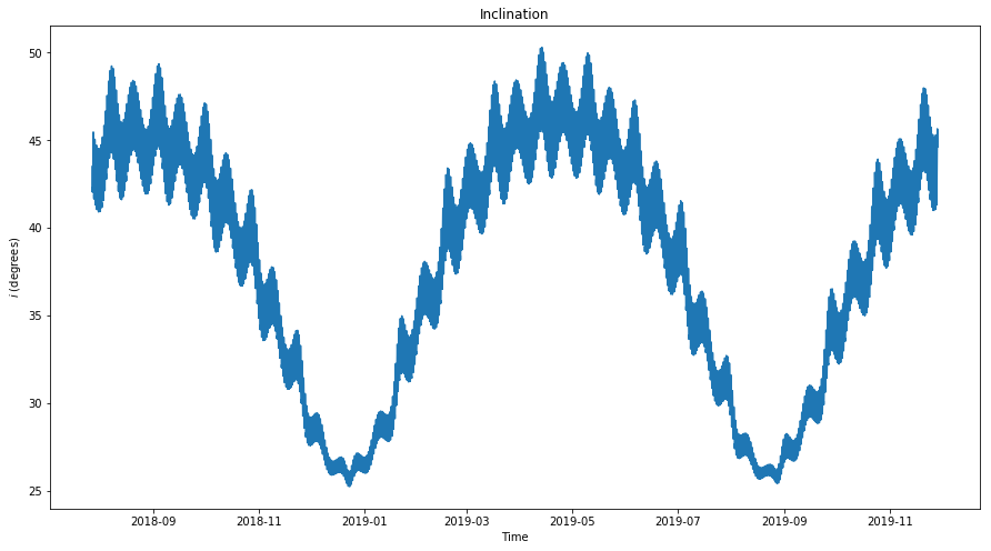
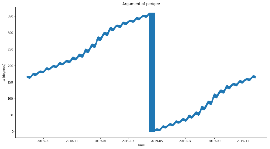
For the case of DSLWP-B’s orbit, the parameters \(i\) and \(\omega\) are shown below. We see that \(i\) oscillates about a middle value of 35º with an amplitude of 10º and a period of 8 months. The argument of periapsis \(\omega\) is monotone increasing with roughly a constant slope and completes a full revolution in 16 months.
Since the values of \(e\) and \(i\) do not change a lot for DSLWP-B, we can replace them by constant average values \(e_0\) and \(i_0\) in the expressions above to obtain simplified models that give the same qualitative behaviour.
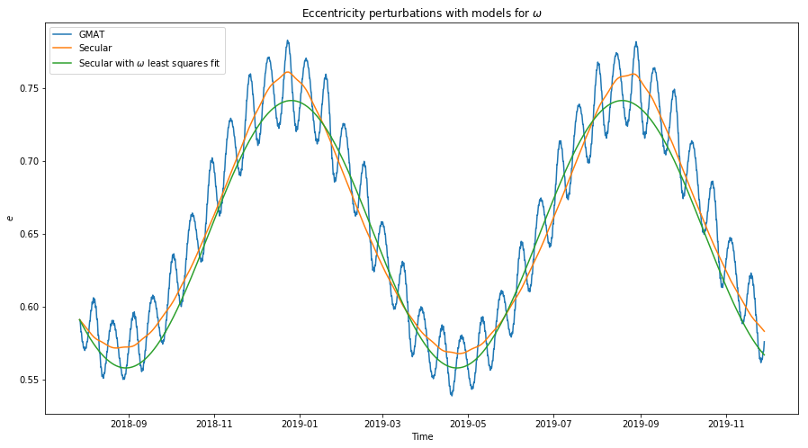
The figure below shows the model for the perturbations of the eccentricity of DSLWP-B. The complete model with long period and secular perturbations has been computed using (1) with \(e\) replaced by \(e_0 = 0.67\). The model for secular perturbations has been computed using (2) with \(e\) replaced by \(e_0\) and \(i\) replaced by \(i_0 = 0.64\) radians.
The model for the secular perturbations of the eccentricity we are using reduces to\[e(t) = e(0) + 10C e_0 \sqrt{1-e_0^2} \sin^2 i_0 \int_0^t \sin 2\omega(\tau)\,d\tau.\]Thus, the behaviour of \(\omega\) governs the secular evolution of the eccentricity. If we are able to approximate \(\omega\) as \(\omega(\tau) = \alpha_0 + \alpha_1 \tau\) then\[e(t) = e(0) – \frac{10C}{\alpha_1} e_0 \sqrt{1-e_0^2} \sin^2 i_0 (\cos(2 \alpha_0 + \alpha_1 t) – \cos(2 \alpha_0)),\]so the secular evolution of the eccentricity is a sinusoid with period \(2\pi/\alpha_1\).
Therefore, we are lead to the study of the secular evolution of the argument of periapsis \(\omega\). However, this is not as easy as the study of the eccentricity. Since in our case \(\omega\) is a monotone function, any error in the approximation of \(\delta\omega\) will tend to accumulate and make the model diverge from the real function when integrating. In this sense, oscillating functions are more tolerant to a small error in the approximation of their derivative.
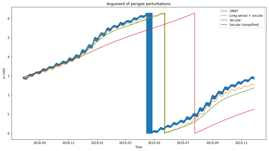
In the figure below we show several models for \(\omega\) compared with the value obtained with GMAT. The most detailed includes long period and secular perturbations and comes directly from (1). Here the actual values for \(e\) and \(i\) have been used. The only value that has been replaced by its average is \(\|r_1\|\), the Earth-Moon distance. The improvement obtained by considering the actual value of \(\|r_1\|\) is very small because the Earth-Moon distance is averaged out over the course of each lunar month, so in all this post we always use the average Earth-Moon distance.
The next model is the secular model taken from (2), again using actual values for \(e\) and \(i\). The least detailed model uses the average values \(e_0\) and \(i_0\), and only the actual value for \(\omega\).
We see that all of these models diverge from the true solution, as they underestimate the growth of \(\omega\). It is interesting that replacing \(e\) and \(i\) by \(e_0\) and \(i_0\) produces increases the error a lot, while in the model for \(e\) it didn’t.
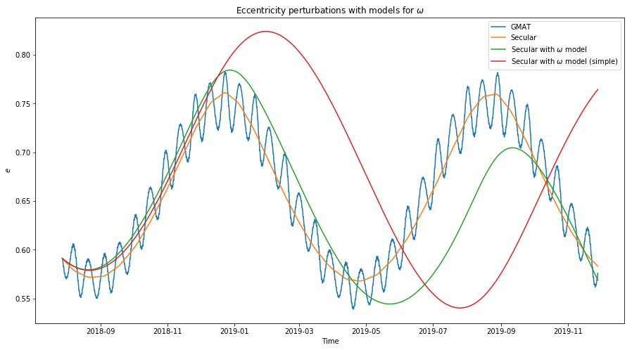
Since the models for the perturbation of \(\omega\) diverge from the true solution, they are not very useful to estimate the secular perturbations of the eccentricity. The figure below shows a comparison between the model of secular perturbations using the actual value of \(\omega\) (orange) and the perturbations using the models given in green and red in the figure above (they are also shown in the same colour below). We see that the period and amplitude of the perturbations predicted by these models are wrong, specially in the case of the simplified model (red).
Since \(\omega\) grows almost linearly, an interesting idea to model it is to perform a least squares fit of a polynomial of degree one to the actual data and use that polynomial as a model in the calculation of the perturbations of \(e\). The figure below shows the least squares fit. As you can see, the fit is quite good.
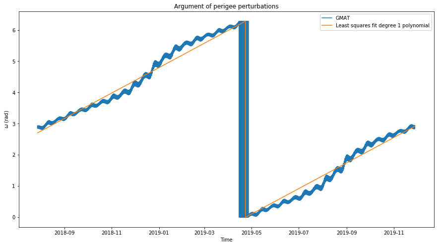
The least squares fit has a slope of 0.0133 radians per day. This means that half a revolution is completed in 236 days, or 7.87 months. This is also the period of the secular perturbations of the eccentricity.
The model for the secular perturbations of \(e\) using the least squares fit for \(\omega\) is shown below. We see that it gives quite a good model. The amplitude and period are close the actual ones.
Next we study the ascending node \(\Omega\). Note that in the rotating coordinate frame we are using, \(\Omega\) has the form \(\Omega = \Omega_0 – \lambda_1 t\), where \(\Omega_0\) is slowly varying and \(\lambda_1\) is the angular velocity of the rotation of the Moon around the Earth, since the \(x\) axis always points to the Earth. Therefore, we plot and model \(\Omega + \lambda_1 t\) instead of \(\Omega\).
Below we show the model for long period and secular perturbations, obtained from (1) using the actual values for \(\omega\), \(i\) and \(e\), and the model for secular perturbations, obtained from (2) again with the actual values for \(\omega\), \(i\) and \(e\).
We note two things: first, as in the case of the argument of periapsis \(\omega\), the models diverge slightly from the actual values obtained in GMAT; second, there are some erratic oscillations in the actual value of \(\Omega\) that are not predicted by the long period perturbation model. I do not know the cause of this effect. Perhaps it is caused by higher order terms in the gravitational force of Earth (recall that here we are using a first order approximation).
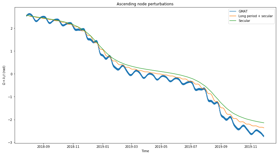
Since the value of \(\Omega\) is not used in the models for the secular perturbations, we do not try to find a better model for \(\Omega\) as we have done for \(\omega\).
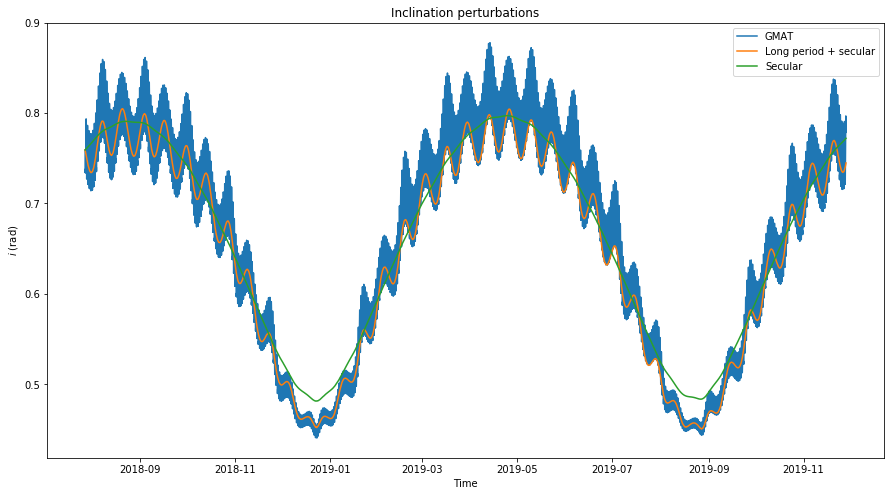
Below we show the models for the inclination \(i\). The long period and secular perturbations model is obtained from (1) using actual values for \(\omega\), \(i\), and \(e\). The secular model is obtained from (2) using only the actual value for \(\omega\). The averages \(i_0\) and \(e_0\) are used instead of \(i\) and \(e\) respectively. We see that these two models are a good match with the actual data.
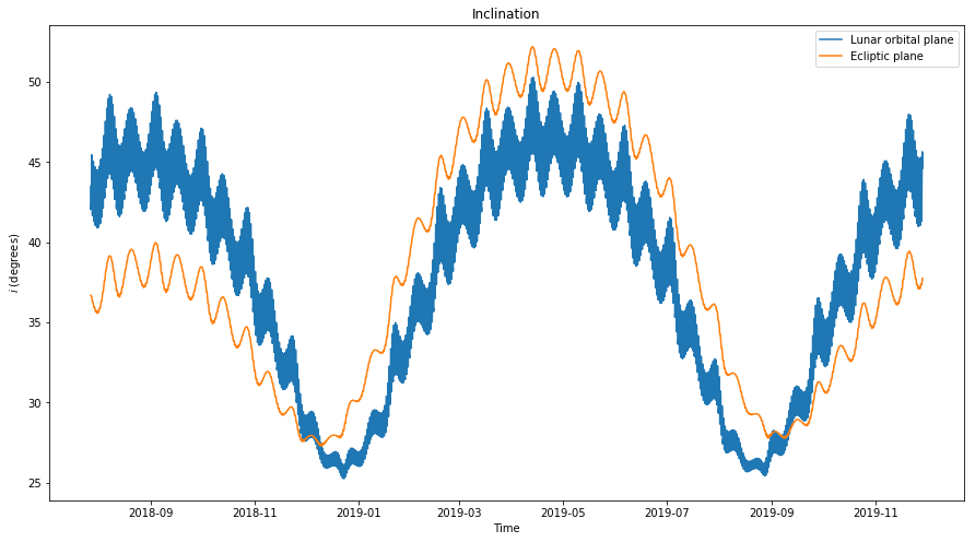
It is interesting to compare the inclination with respect to the lunar orbital plane (which is the variable \(i\) we are considering here) versus the inclination with respect to the ecliptic plane (which is usually considered as the reference plane in a lunar inertial reference frame). Since the lunar orbital plane is inclined 5.14º with respect to the ecliptic, we see that depending on the position of the ascending node, both inclinations will differ by up to \(\pm\)5.14º.
This causes that the inclination, when viewed with respect to the lunar orbital plane has a regular behaviour with more or less the same period as the eccentricity (owing to the term \(\sin 2\omega\) in (2)), but when viewed with respect to the ecliptic plane the behaviour is more complicated, since the time that takes \(\Omega_0\) to make a full revolution is not related to this period. The effect is more visible when the inclination is plotted for several years (see this post).
For the accumulated long periodic perturbations of \(e\), El’Yasberg’s book gives the following formula\[
\tilde{\delta e} = \frac{15}{16}\frac{\mu_1}{\mu_0}\left(\frac{a}{\|r_1\|}\right)^3\frac{P_1}{P}D(\omega, i)e\sqrt{1-e^2}
[\cos(2\Omega + \varphi) – \cos(2\Omega_0 + \varphi_0)],\]where\[
D(\omega,i) = \sqrt{4\cos^2 i \cos^2 2\omega + (1+\cos^2i)^2 \sin^2 2\omega},\]
and \(\varphi\) is defined by\[\cos\varphi = \frac{2\cos i \cos 2\omega}{D(\omega,i)},\ \sin\varphi = \frac{(1+\cos^2i)\sin 2\omega}{D(\omega,i)}.\] Note that \(\tilde{\delta e}\) is not the increment in \(e\) per revolution, but rather the total increment from the time \(t_0=0\) to a certain time \(t\) where all the parameters are evaluated. Here \(\Omega_0\) and \(\varphi_0\) stand for \(\Omega\) evaluated at time \(t = 0\).
The figure below shows the actual eccentricity, as simulated in GMAT, the model for the long periodic perturbations, which is taken from the equation above with \(e_0\) instead of \(e\), and the GMAT data with the secular perturbations removed. We see that the model is a good match.
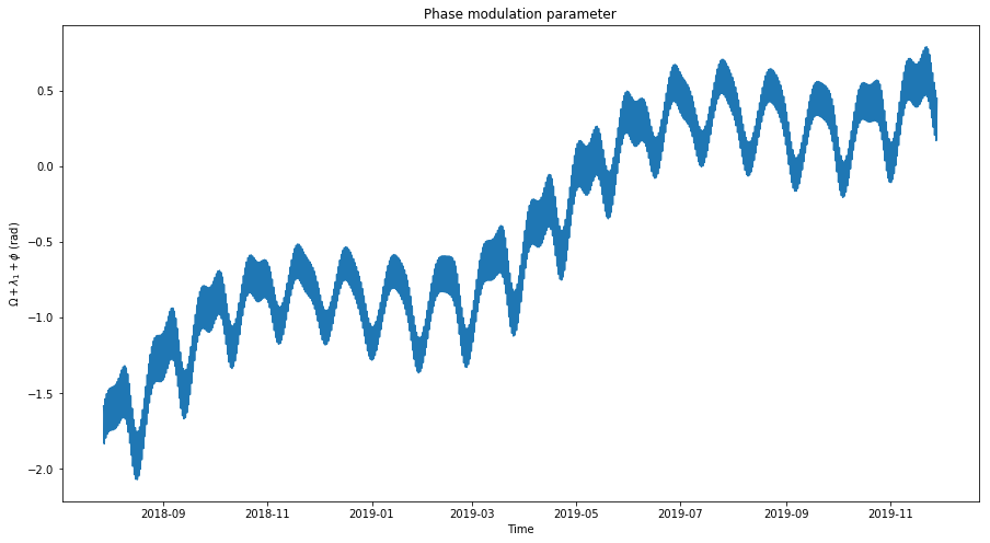
If we write \(2\Omega + \varphi = -2\lambda_1t + [\Omega + \lambda_1 t + \varphi]\) and denote by \(\psi\) the term in brackets, we see that \(\psi\) is slowly varying. Therefore, the behaviour of \(\tilde{\delta}{e}\) is a sinusoidal of period \(P_1/2\) which is phase modulated by the slowly varying parameter \(\psi\). The figure below shows the evolution of the phase modulating parameter \(\psi\).
The calculations for this post have been made in this Jupyter notebook. The GMAT script with the orbital simulation can be found here.
One comment