DSLWP-B and the lunar eclipse

As you may well know, last Friday 27th July there was a total lunar eclipse. This is an interesting event for lunar-orbiting spacecraft such as DSLWP-B. In fact, depending on the spacecraft’s orbit, it may also pass through the Earth’s umbra or penumbra. Here I look at the trajectory taken by DSLWP-B during the eclipse.

Comparison of DSLWP-B orbit determination with tracking files

In the last post I compared the results of my orbit determination for DSLWP-B using one lunar month of Doppler data with the observations in the VLBI experiment done on June 10. In this post I will compare my orbit determination with the tracking files published by Wei Mingchuan BG2BHC in gr-dslwp. These tracking files are produced from the orbit determination performed by the Chinese Deep Space Network using two-way S-band Doppler measurements.

The tracking files contain a listing of the position \(x\) and velocity \(v\) vectors for DSLWP-B in ECEF coordinates. The entries are given at intervals of one second. The tracking files can be used directly to compute Doppler as received in a groundstation. In fact, if the ECEF coordinates of the groundstation are \(x_0\), then \(R = \langle x – x_0, v\rangle/\|x-x_0\|\) is the range-rate, and so the Doppler can be computed as \(D=-fR/c\), where \(f\) is the downlink frequency and \(c\) is the speed of light in vacuum. Here I have used this method to compute the Doppler according to the tracking files.

All the tracking files published so far have been considered in this study, except for the first two, which contained an incorrect anomaly at epoch. The figure below shows the residuals between the Doppler measurements made by Scott Tilley VE7TIL and my orbit determination (called “new elements”) and each of the tracking files. It seems that the residuals are quite similar.

The figure below shows the difference between the Doppler according to each of the tracking files and the Doppler predicted by my orbit determination.

It seems that the match is quite good for the central days, but not so good towards the edges. My orbit determination is numerically propagated from a single set of elements at MJD 28264.5 for the whole period, while the tracking files probably use different sets of elements that are propagated numerically over a few days only. Therefore it might happen that my orbit determination is affected by some accumulative error due to numerical integration or an inaccuracy in the force model.

Validation of DSLWP-B orbit determination using VLBI observations

In my last post I presented my orbit determination of DLSWP-B using one lunar month of S-band Doppler measurements made by Scott Tilley VE7TIL. In this post, I will use the delta-velocity measurements from the VLBI experiment on 2018-06-10 to validate my orbital elements.

In the figures below, I compare between the sets of data: The old elements, obtained in this post:

DSLWP_B.SMA = 8762.40279943
DSLWP_B.ECC = 0.764697135746
DSLWP_B.INC = 18.6101083906
DSLWP_B.RAAN = 297.248156986
DSLWP_B.AOP = 130.40460851
DSLWP_B.TA = 178.09494681

The new elements obtained in my last post:

DSLWP_B.SMA = 8765.95638789
DSLWP_B.ECC = 0.764479041563
DSLWP_B.INC = 23.0301858287
DSLWP_B.RAAN = 313.64185464
DSLWP_B.AOP = 113.462338342
DSLWP_B.TA = 178.5519212

The elements obtained from the 20180610 tracking file published by Wei Mingchuan BG2BHC in dslwp_dev. This tracking file contains a list of ECEF position and velocity vectors for DSLWP-B. The first entry is taken as the orbital state and the orbit is propagated in GMAT, as done in this post. It would also be possible to calculate the delta-velocity directly from the ECEF data, but the results would be fairly similar and I already have a script to do it with GMAT orbit propagation.

A degree 2 polynomial fit to the VLBI observations. It turns out that the delta-velocity during the VLBI experiment can be approximated fairly well by a parabola, so it makes sense to use this as a reference. Note that this also implies that this set of delta-velocity measurements alone would be insufficient to perform orbit determination, as a degree 2 polynomial gives us 3 coefficients, while we would need to determine 6 parameters for the orbital state. Adding delta-range would only give us an extra variable, so orbit determination using VLBI would need several sets of measurements well space in time so that the orbit can be observed at different anomalies.

The figures below show a comparison between the four sets of data and the VLBI measurements.

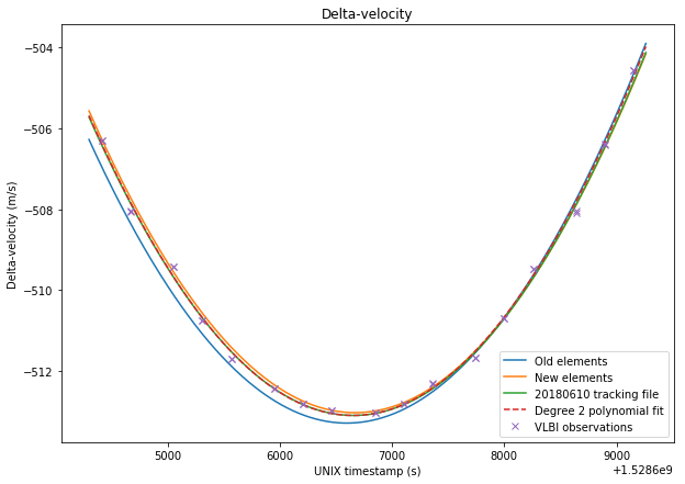
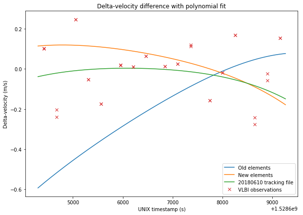
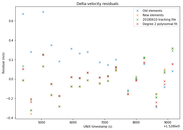
The RMS errors are respectively 0.248m/s for the old elements, 0.167m/s for the new elements, 0.156m/s for the tracking file, and 0.137m/s for the polynomial fit. Thus, we see that the newer elements represent a good improvement over the older elements. The tracking file gives a slightly better result than the new elements. However, the new elements should give good results over a long time span of over 20 days, as we have seen in the previous post, while the orbital parameters derived from the tracking files tend to change often.

The Jupyter notebook used to make these calculations has been updated in here.

DSLWP-B first month in orbit

DSLWP-B has now been for more than a month in lunar orbit, since the orbital injection was made on May 25. Scott Tilley VE7TIL has sent me his latest batch of S-band Doppler measurements, including data for all this first lunar month. Having a complete lunar month of data is interesting for orbit determination purposes, since it gives observability of the orbit from all possible right ascension angles.
I have run my orbit determination with the new data.

Update on DSLWP-B orbit determination

Last Sunday, I used Scott Tilley VE7TIL’s Doppler measurements of the DSLWP-B S-band beacon to perform orbit determination using GMAT. Yesterday Scott sent me the Doppler data he has been collecting during this week. I have re-run my orbit determination process to include this new data.

Below I show the Keplerian state that was determined on 2018-06-03, in comparison with the new state determined on 2018-06-10 (both are referenced to the same epoch of 2018-05-26 00:00:00 UTC).

% 20180603
%DSLWP_B.SMA = 8761.0758581
%DSLWP_B.ECC = 0.768016853537
%DSLWP_B.INC = 16.9728174682
%DSLWP_B.RAAN = 295.670653562
%DSLWP_B.AOP = 130.427472407
%DSLWP_B.TA = 178.126596496

% 20180610
DSLWP_B.SMA = 8762.40279943
DSLWP_B.ECC = 0.764697135746
DSLWP_B.INC = 18.6101083906
DSLWP_B.RAAN = 297.248156986
DSLWP_B.AOP = 130.40460851
DSLWP_B.TA = 178.09494681

It seems that there is still an indetermination of a few degrees in the inclination and right-ascension of the ascending node and a few kilometres in the semi-major axis.

The graph below shows the Doppler fit.

The Jupyter notebook where these calculations are performed can be found here.

DSLWP-B’s journey to the Moon: part III

This is a follow-up on the series about DSLWP-B’s orbital dynamics (see part I and part II). In part I we looked at the tracking files published by Wei Mingchuan BG2BHC, which list the position and velocity of the satellite in ECEF coordinates, and presented basic orbit propagation with GMAT. In part II we explored GMAT’s capabilities to plan and perform manoeuvres, making a tentative simulation of DSLWP-B’s mid-course correction and lunar orbit injection. Now we turn to the study of DSLWP-B’s elliptical lunar orbit.

In this post we will examine the Keplerian elements of the orbits described by each of the tracking files published so far. We will also use Scott Tilley VE7TIL’s Doppler measurements of the S-band beacon of DSLWP-B to validate and determine the orbit.

DSLWP-B’s journey to the Moon: part II

This forms parts of a series of posts showing how to use GMAT to track the DSLWP-B Chinese lunar satellite. In part I we looked at how to examine and validate the tracking files published by BG2BHC using GMAT. It is an easy exercise to use GMAT to perform orbit propagation and produce new tracking files. However, note that the available tracking files come from orbit planning and simulation, not from actual measurements. It seems that the elliptical lunar orbit achieved by DSWLP-B is at least slightly different from the published data. We are already working on using Doppler measurements to perform orbit determination (stay tuned for more information).

Recall that there are three published tracking files that can be taken as a rough guideline of DSLWP-B’s actual trajectory. Each file covers 48 hours. The first file starts just after trans-lunar injection, and the second and third files already show the lunar orbit. Therefore, there is a gap in the story: how DSLWP-B reached the Moon.

There are at least two manoeuvres (or burns) needed to get from trans-lunar injection into lunar orbit. The first is a mid-course correction, whose goal is to correct slightly the path of the spacecraft to make it reach the desired point for lunar orbit injection, which is usually the lunar orbit periapsis (the periapsis is the lowest part of the elliptical orbit). The second is the lunar orbit injection, a braking manoeuvre to get the spacecraft into the desired lunar orbit and adjust the orbit apoapsis (the highest part of the orbit). Without a lunar orbit injection, the satellite simply swings by the Moon and doesn’t enter lunar orbit.

In this post we will see how to use GMAT to calculate and simulate these two burns, so as to obtain a full trajectory that is consistent with the published tracking files. The final trajectory can be seen in the figure below.

DSLWP-B orbit from trans-lunar injection to lunar orbit injection and elliptical orbit

DSLWP-B’s journey to the Moon: part I

As you may well know, on May 20 a CZ-4C rocket launched from Xichang, China, to deliver Queqiao, the Chang’e 4 relay satellite, to the Moon. Queqiao is a communications relay satellite designed to orbit the L2 point of the Earth-Moon system, supporting the future Chang’e 4 rover that will land on the far side of the Moon. From the L2 point, Queqiao has a good view of both the Earth and the far side of the Moon.

This launch was shared by the DSLWP-A and -B microsatellites, also called Longjiang 1 and 2. These two satellites are designed to be put on a 200 x 9000km lunar orbit and their main scientific mission is a proof of concept of the Discovering the Sky at Longest Wavelengths experiment, a radioastronomy HF interferometer that uses the Moon as a shield from Earth’s interferences.

The DSLWP satellites carry an Amateur radio payload which consists of a 250 baud (or 500 baud) GMSK transmitter which uses \(r=1/2\) or \(r=1/4\) turbo codes, a JT4G beacon, and a camera allowing open telecommand (such as the camera on BY70-1 and LilacSat-1). A year ago, while the radio system was being designed, I wrote a post about DSLWP’s SSDV downlink, which transmits the images taken by the camera.

Wei Mingchuan BG2BHC, who is part of the DSLWP team, has been posting updates on Twitter about the status of the mission. If you’ve been following these closely, you’ll already know that unfortunately radio contact with DSLWP-A was lost on the UTC afternoon of May 22. Since then, all tries to contact the spacecraft have failed (the team will publicly release more information about its fate soon). On the other hand, DSLWP-B has been successfully injected into lunar orbit and is now orbiting the Moon since the UTC afternoon of May 25.

More posts will follow about the radio communications of DSLWP, but this series of posts will deal with the orbital dynamics part of the mission. In this first post, I will look at the tracking files released so far by Wei, which can be used to compute the spacecraft’s position and Doppler.

A brief study of TLE variation

During my research and experiments about using WSJT-X modes through linear transponder satellites, one of the questions I had is by how much do TLEs of different epochs for the same satellite vary. This was glimpsed in part II, where I plotted the “best delay” parameter for TLEs of different age.

The topic of accuracy in TLE computation and propagation is rather complex. A NORAD TLE is the result of an orbit determination after several radar measurements at different epochs, so the elements are in some sense “averaged” over time. Also, the SGP4 propagator is simple and doesn’t model many orbit perturbations. However, NORAD TLEs are specially crafted to give improved results when used with SGP4.

Nevertheless, here I present a simple way of studying the rate of change of NORAD TLEs at different epochs. This procedure might not be very meaningful or sophisticate, but still seems to yield some interesting results.