This forms parts of a series of posts showing how to use GMAT to track the DSLWP-B Chinese lunar satellite. In part I we looked at how to examine and validate the tracking files published by BG2BHC using GMAT. It is an easy exercise to use GMAT to perform orbit propagation and produce new tracking files. However, note that the available tracking files come from orbit planning and simulation, not from actual measurements. It seems that the elliptical lunar orbit achieved by DSWLP-B is at least slightly different from the published data. We are already working on using Doppler measurements to perform orbit determination (stay tuned for more information).
Recall that there are three published tracking files that can be taken as a rough guideline of DSLWP-B’s actual trajectory. Each file covers 48 hours. The first file starts just after trans-lunar injection, and the second and third files already show the lunar orbit. Therefore, there is a gap in the story: how DSLWP-B reached the Moon.
There are at least two manoeuvres (or burns) needed to get from trans-lunar injection into lunar orbit. The first is a mid-course correction, whose goal is to correct slightly the path of the spacecraft to make it reach the desired point for lunar orbit injection, which is usually the lunar orbit periapsis (the periapsis is the lowest part of the elliptical orbit). The second is the lunar orbit injection, a braking manoeuvre to get the spacecraft into the desired lunar orbit and adjust the orbit apoapsis (the highest part of the orbit). Without a lunar orbit injection, the satellite simply swings by the Moon and doesn’t enter lunar orbit.
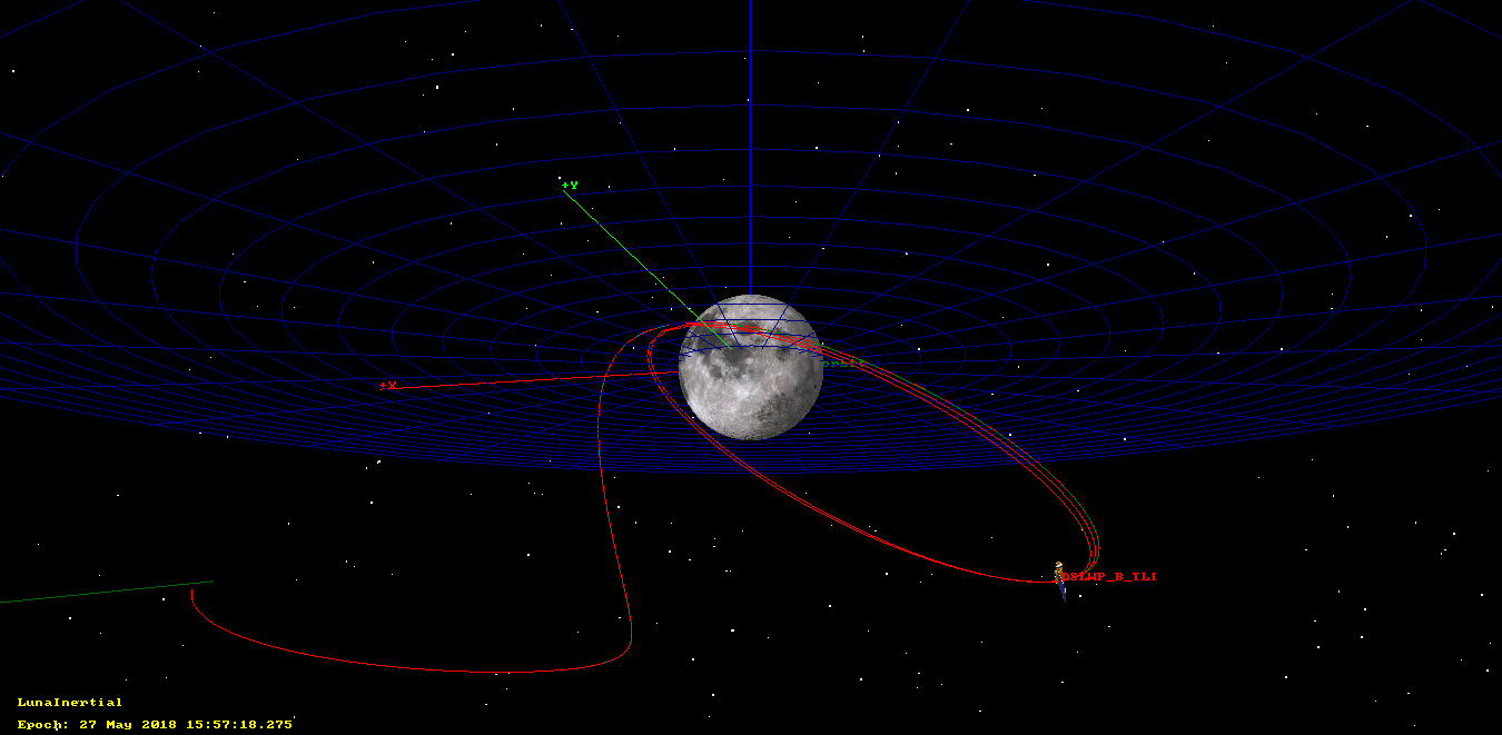
In this post we will see how to use GMAT to calculate and simulate these two burns, so as to obtain a full trajectory that is consistent with the published tracking files. The final trajectory can be seen in the figure below.
We have very few data (either from planning or from real measurements) regarding the burns performed by DSLWP-B. We know the following:
- The trajectory following trans-lunar injection
- The lunar elliptical orbit after lunar orbit injection
- A tentative date for the mid-course correction: 22 May 2018 22:55:00 UTC (but it seems that the correction was delayed)
- Some information by Nico Janssen PA0DLO regarding lunar orbit injection: “On 2018-05-25 between 14:00 and 15:00 UTC they are expected to pass the Moon at a distance of about 300 km. At that time they should perform a braking maneuver so that they can enter a high elliptical 300 x 9000 km orbit around the Moon.”
- The confirmation forwarded by PA0DLO that DSLWP-B achieved lunar orbit, sent at 16:25 UTC.
The rest of the details are still unknown. Therefore we will use our imagination and plan some manoeuvres that more or less agree with the available data and look plausible. If we learn further details we can always modify and refine our calculations.
The GMAT script I’ve used for this post is available in dslwp_injection.script. I have written it partly by hand, partly with help of the GUI. Here I will explain some of the more important sections of this script. It is recommended that you take a look at the target Mars B-plane tutorial to become familiar with the techniques I will use.
The idea of the calculations in this script goes as follows. We will use two elements for DSLWP-B: the start of the first tracking file (just after trans-lunar injection) and the start of the second tracking file (already in lunar orbit). We will perform a burn at 22 May 2018 22:55:00 to get at the appropriate time into the lunar periapsis given by the elliptical lunar orbit described by the second tracking file. Then we will perform a lunar orbit injection to match completely the elliptical lunar orbit. Note that orbit injections are usually done at periapsis because of the Oberth effect.
To do the required calculations, we will first propagate backwards in time the start of the second tracking file until the spacecraft reaches lunar periapsis, and we will take note of the epoch \(t_P\), position \(x_P\) and velocity \(v_P\) of the spacecraft. Then, we will take the start of the first tracking file and propagate forwards in time until the mid-course correction at 2018-05-22 22:55:00. We will then calculate a burn that makes the spacecraft reach the periapsis position as we have noted before (at the epoch \(t_P\), the position should be \(x_P\)). Finally, the lunar orbit injection burn is calculated to make the velocity of the spacecraft match \(v_P\).
In the GMAT script file, first we create the two spacecraft that we will use in the calculations. The first represents the start of the first tracking file and the second represents the start of the second file. We also include the mass of the satellite, which is known to be 45kg, and approximate values for the parameters used for solar radiation pressure and atmospheric drag calculations.
% Initial element from program_tracking_dslwp-a_20180520_window1.txt
% DSLWP-B after trans-lunar injection
Create Spacecraft DSLWP_B_TLI
DSLWP_B_TLI.DateFormat = UTCModJulian
DSLWP_B_TLI.Epoch = '28259.413090277776'
DSLWP_B_TLI.CoordinateSystem = EarthFixed
DSLWP_B_TLI.X = -6633.271172
DSLWP_B_TLI.Y = -802.293973
DSLWP_B_TLI.Z = -538.972574
DSLWP_B_TLI.VX = 0.029033
DSLWP_B_TLI.VY = -9.016021
DSLWP_B_TLI.VZ = -5.164087
DSLWP_B_TLI.DryMass = 45
DSLWP_B_TLI.Cd = 2.2
DSLWP_B_TLI.Cr = 1.8
DSLWP_B_TLI.DragArea = 0.25
DSLWP_B_TLI.SRPArea = 0.25

% Initial element from program_tracking_dslwp-b_20180526.txt
% DSLWP-B in lunar orbit
Create Spacecraft DSLWP_B_orbit
DSLWP_B_orbit.DateFormat = UTCModJulian
DSLWP_B_orbit.Epoch = '28264.5'
DSLWP_B_orbit.CoordinateSystem = EarthFixed
DSLWP_B_orbit.X = 303527.4363
DSLWP_B_orbit.Y = -255336.4971
DSLWP_B_orbit.Z = -38291.07068
DSLWP_B_orbit.VX = -17.836844
DSLWP_B_orbit.VY = -21.171093
DSLWP_B_orbit.VZ = -0.471039
DSLWP_B_orbit.DryMass = 45
DSLWP_B_orbit.Cd = 2.2
DSLWP_B_orbit.Cr = 1.8
DSLWP_B_orbit.DragArea = 0.25
DSLWP_B_orbit.SRPArea = 0.25
The GMAT mission script begins by setting the variable correctionEpoch with the epoch for the mid-course correction. We also set an initial guess for the delta-v corresponding to this correction. This guess is actually the correct solution, which has been found before by running the script. At first, we knew nothing about the correct solution, so we set an initial guess of zero. The GMAT solver then finds the solution by starting with our guess and trying several values until it finds one that works. By storing that solution and using it as our initial guess, we save many computations when running the mission script again. It is an easy exercise for the reader to set the initial guess to zero again and see what happens.
BeginMissionSequence;
BeginScript 'Init'
   correctionEpoch = 28261.45486111111 % 22 May 2018 22:55:00 UTC
EndScript

BeginScript 'Correction initial guesses'
   Correction.Element1 = 0.0135414468457
   Correction.Element2 = -0.0278871540458
   Correction.Element3 = -0.0145043816337
EndScript
As we have described above, we propagate the spacecraft in lunar orbit backwards in time until it reaches the periapsis. Then we propagate the spacecraft in trans-lunar injection forward in time until the mid-course correction epoch. The PenUp and PenDown commands are used to avoid discontinuities in the plots, since we are jumping in time.
% Propagate Luna orbit back to periapsis
Propagate BackProp LunaProp(DSLWP_B_orbit) {DSLWP_B_orbit.Luna.Periapsis}

% Propagate from Earth to mid-course correction
PenUp EarthLunaView LunaOrbitView
Propagate EarthProp(DSLWP_B_TLI) {DSLWP_B_TLI.ElapsedSecs = 60} % this is to avoid jumps in the plots
PenDown EarthLunaView LunaOrbitView
Propagate EarthProp(DSLWP_B_TLI) {DSLWP_B_TLI.UTCModJulian = correctionEpoch}
The next part of the mission script calculates the appropriate mid-course correction epoch using a DC (Differential Corrector) solver. Here we use the solver to try different values for the correction delta-v, then perform the manoeuvre and propagate until the epoch when the spacecraft should reach the lunar periapsis. We impose that at this moment the position of both satellites must coincide.
Target 'Target lunar periapsis' DC
   % Vary mid-course correction parameters
   Vary DC(Correction.Element1 = Correction.Element1, {Perturbation = 0.0001, MaxStep = 0.005})
   Vary DC(Correction.Element2 = Correction.Element2, {Perturbation = 0.0001, MaxStep = 0.005})
   Vary DC(Correction.Element3 = Correction.Element3, {Perturbation = 0.0001, MaxStep = 0.005})

   % Perform mid-course correction
   Maneuver 'Mid-course correction' Correction(DSLWP_B_TLI)

   % Propagate to epoch of lunar periapsis
   Propagate LunaProp(DSLWP_B_TLI) {DSLWP_B_TLI.UTCModJulian = DSLWP_B_orbit.UTCModJulian}

   % Impose conditions of arrival to periapsis
   Achieve DC(DSLWP_B_TLI.X = DSLWP_B_orbit.X, {Tolerance = 0.001})
   Achieve DC(DSLWP_B_TLI.Y = DSLWP_B_orbit.Y, {Tolerance = 0.001})
   Achieve DC(DSLWP_B_TLI.Z = DSLWP_B_orbit.Z, {Tolerance = 0.001})
EndTarget
When we have found the appropriate mid-course correction, we write the parameters to a report file for later analysis. Then, we compute the lunar orbit injection delta-v. Since the condition for this burn is that both spacecrafts should end up with the same velocity vector, the delta-v is straightforward to compute as the difference in velocities. Here we are using the DSLWP_B_TLI_VBN reference frame, which is a V (velocity), N (normal), B (binormal) reference frame to be explained below. We are only using this frame to interpret the results more easily. Any other reference frame would be adequate.
Once the delta-v has been computed, we perform the manoeuvre, write the parameters to the report file and then propagate for 2 days to see that the orbit we have achieved really matches the orbit described in the second tracking file.
Report 'Report mid-course correction burn' burnsReport correctionEpoch Correction.Element1 Correction.Element2 Correction.Element3

BeginScript 'Setup LOI'
    LOI.Element1 = DSLWP_B_orbit.DSLWP_B_TLI_VNB.VX - DSLWP_B_TLI.DSLWP_B_TLI_VNB.VX
    LOI.Element2 = DSLWP_B_orbit.DSLWP_B_TLI_VNB.VY - DSLWP_B_TLI.DSLWP_B_TLI_VNB.VY
    LOI.Element3 = DSLWP_B_orbit.DSLWP_B_TLI_VNB.VZ - DSLWP_B_TLI.DSLWP_B_TLI_VNB.VZ
EndScript

Maneuver 'Lunar orbit injection 'LOI(DSLWP_B_TLI)

Report 'Report LOI burn' burnsReport DSLWP_B_TLI.UTCModJulian LOI.Element1 LOI.Element2 LOI.Element3

Propagate LunaProp(DSLWP_B_TLI) {DSLWP_B_TLI.ElapsedDays = 2}
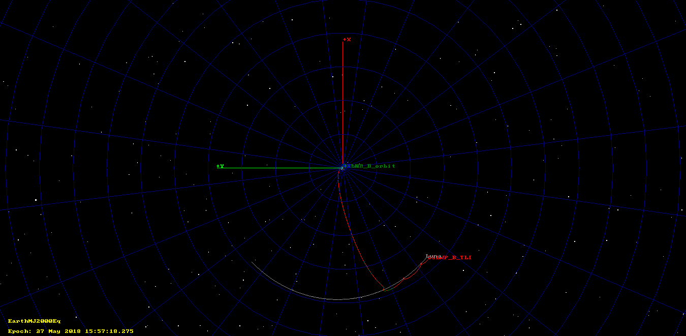
Below we can see the final trajectory in an ECI reference frame.
The VNB (velocity-normal-binormal) frame is a very usual reference frame to plan orbital manoeuvres. It is centred on the spacecraft and its three coordinate vectors point as follows: the V vector points along the velocity vector, tangent to the orbit; the N vector is perpendicular to V and contained in the orbital plane; the B vector completes a right-handed coordinate system. Burns along the V vector increase or decrease the orbital speed, changing the eccentricity and semi-major axis, and burns along the B vector change the orbital plane. Therefore, it is easy to understand what is the effect of a particular burn in terms of its expression in the VNB frame. For that reason, we have used VNB frames for both burns.
For the lunar orbit injection burn, we need to do calculations (compute the velocity vector of both spacecraft) in the VNB frame of DSLWP_B_TLI, so we need to declare explicitly this reference frame as follows.
Create CoordinateSystem DSLWP_B_TLI_VNB
DSLWP_B_TLI_VNB.Origin = DSLWP_B_TLI
DSLWP_B_TLI_VNB.Axes = ObjectReferenced
DSLWP_B_TLI_VNB.XAxis = V
DSLWP_B_TLI_VNB.YAxis = N
DSLWP_B_TLI_VNB.Primary = Luna
DSLWP_B_TLI_VNB.Secondary = DSLWP_B_TLI
After running the script, the contents of the burns report file (stored in output/burnsReport.txt) is the following:
correctionEpoch           Correction.Element1       Correction.Element2       Correction.Element3
28261.45486111111         0.0135414468457           -0.0278871540458          -0.0145043816337
DSLWP_B_TLI.UTCModJulian   LOI.Element1              LOI.Element2              LOI.Element3
28264.16954021541          -0.2951585933116597       0.001252079927705898      0.04183219943959633
The units of the burn elements are km/s. We see that the mid-course correction is a small burn, with a total delta-v of 34.2 m/s. The lunar-orbit injection is a much larger burn, with a total delta-v of 298.1 m/s. Most of the burn happens in the retrograde (-V) direction. This is because the spacecraft is braked to enter lunar orbit.
The epoch of the lunar orbit insertion, which coincides with the lunar periapsis immediately before 2018-05-26 00:00:00 UTC, is 2018-05-25 16:04:08 UTC. This seems a little late, given the reports by Nico that lunar orbit injection would be around 14:00 or 15:00, and the confirmation of successful orbit injection at 16:25.
The altitude of the periapsis can be seen by using the “Command summary” feature of GMAT, just after the lunar orbit injection burn. It is 368.27km, which matches more or less Nico’s information. Other interesting orbital parameters (in the lunar inertial reference frame) are as follows.
- Orbit period: 73455s (20h 24min 15s)
- Semi-major axis: 8750.7km
- Eccentricity: 0.759
- Inclination: 20.8º
- Right-ascension of ascending node: 308.2º
- Argument of perigee: 118º
- Altitude of apoapsis: 13655km
The burns we have performed in GMAT are impulsive burns, where the velocity is changed instantly. This is not realistic but makes burn planning easier. Some knowledge of the propulsion system of DSLWP-B would enable us to use finite burns, which simulate the finite amount of thrust that is available. Fuel consumption is also modelled.
In this post we have seen how to imagine and plan some plausible manoeuvres with the little data we have available. Additional knowledge would enable us to constrain our freedom and simulate a more realistic trajectory. We would need to have at least some of the following data.
Data regarding the burns:
- Epoch of the mid-course correction
- Delta-v of mid-course correction (as a vector, or total delta-v, or just Doppler change, which represents the projection of the delta-v vector onto the line of sight)
- Epoch of the lunar orbit injection
- Delta-v of the lunar orbit injection
- Whether the lunar orbit injection happened right at periapsis or somewhere near
Data regarding the thruster for DSLWP-B. Among other parameters, GMAT allows to use the following:
- Geometry of the thruster with respect to the spacecraft’s body (thrust direction)
- Thrust and specific impulse, depending on the tank pressure and temperature (see here for details)
Data regarding the fuel tanks for DSLWP-B. GMAT allows us to model the following parameters of a chemical tank:
- Fuel mass
- Fuel density (some estimate using the type of fuel would suffice)
- Temperature and reference temperature (probably not so important)
- Pressure in the fuel tank
- Volume of the fuel tank
- Pressure model: pressure regulated or blow down
With a little luck, we will be able to get some of the data (or at least ballpark estimates) from the DSLWP team and use it to refine our simulations.
3 comments