Yesterday I reported about Tianwen-1’s first trajectory correction manoeuvre, TCM-1. In that post I commented the possibility that the updated state vectors that we saw on the telemetry after TCM-1 might come from a prediction or planning rather than take into account the actual performance of the burn.
The figure below shows the error between the state vectors collected after TCM-1 over the last two days, and a trajectory propagated in GMAT, using the following state vector, which is one of the first received after TCM-1.
[0151059eb9ea] 2020-08-02 00:17:06.711400 100230220.21360767 -106145016.11787066 -45441035.07405791 25.581827920522485 18.240707152437626 8.567874276424218
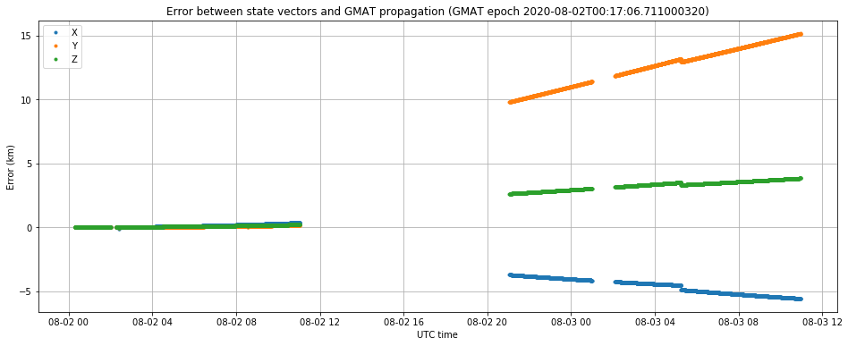
We see that on the UTC night between August 1 and 2 the state vectors deviate very little from the GMAT trajectory. However, on the UTC night between August 2 and 3 we see a slightly different trajectory in the state vectors. We have no data in between, as the spacecraft is not visible in Europe, so we don’t know the precise moment of change. The gap in telemetry around 2020-08-03 00:45 UTC is due to a transmission of high-speed data.
It seems reasonable to think that after TCM-1 the Chinese DSN performed precise ranging of the spacecraft to determine the new orbit accurately and then uploaded a correction to the state vectors on-board Tianwen-1.
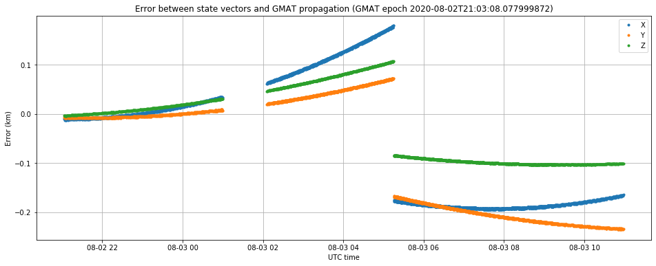
The state vectors from last night all describe the same trajectory, as shown in the plot below which uses
[0151322e67d0] 2020-08-02 21:03:08.078400 102132184.96868199 -104770375.00352533 -44795830.46284772 25.29849580646669 18.532513218789806 8.692135086385246
to propagate a trajectory in GMAT. There is a small jump of a few hundred meters at some point. We usually see one or two these jumps per day, but we don’t understand well why they happen.
The trajectory according to the state vectors from 00:17:06 and from 21:03:08 are very similar. For example, at the closest approach to Mars they only differ in 1197km. For comparison, the difference between the new trajectory and the pre–TCM-1 trajectory is 126529km (again, at the closest approach to Mars).
I have generated a new table of right-ascension, declination and distance coordinates based on the updated state vectors. Note that this table doesn’t include light-time delay to the spacecraft.
Thanks to AMSAT-DL‘s Bochum observatory team and to Paul Marsh M0EYT for their continuous effort in tracking Tianwen-1. The data used in this post has come from their observations.