A month ago I started modifying the GMAT EstimationPlugin to support delta-range observations. This work is needed in order to perform orbit determination with the VLBI observations that we did with DSLWP-B (Longjiang-2) during its mission. Now I have a version which is able to use both delta-range and delta-range rate observations in simulation and estimation. This is pretty much all that’s needed for the DSLWP-B VLBI observations.
The modified GMAT version and accompanying GMAT scripts for this project can be found in the gmat-dslwp Github repository. This post is an account of the work I’ve made.
Simulation and estimation GMAT script
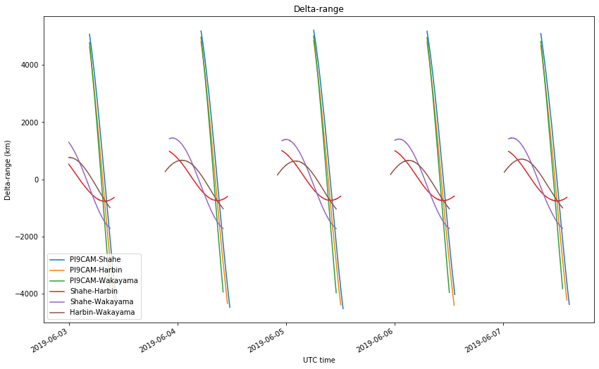
The script simulate-vlbi-june-2019.script is used to showcase all the new functionality. It can be used to simulate the VLBI observations that were done during the first week of June 2019 and then run orbit determination with the simulated observations. The script includes the groundstations of PI9CAM (the Dwingeloo radiotelescope in the Netherlads), Shahe (in Bejing, China), Harbin (China) and Wakayama University (Japan).
The simulation runs between 2019-06-03 and 2019-06-08, which is when the observations were made. It computes the delta-ranges and delta-range rates for all the possible baselines whenever DSLWP-B is in common view of the groundstations. I have made a Jupyter notebook to plot the results of these simulations. The plots can be seen in the figures below.

An error model with the typical noise we saw in the VLBI observations is used for simulation. This has a sigma of 1.2km for delta-range and 0.2m/s for delta-range rate.
For estimation we use AcceptFilter to select only the observations corresponding to the slots when the Amateur payload was active. These are a 2 hour slot on each observation day.
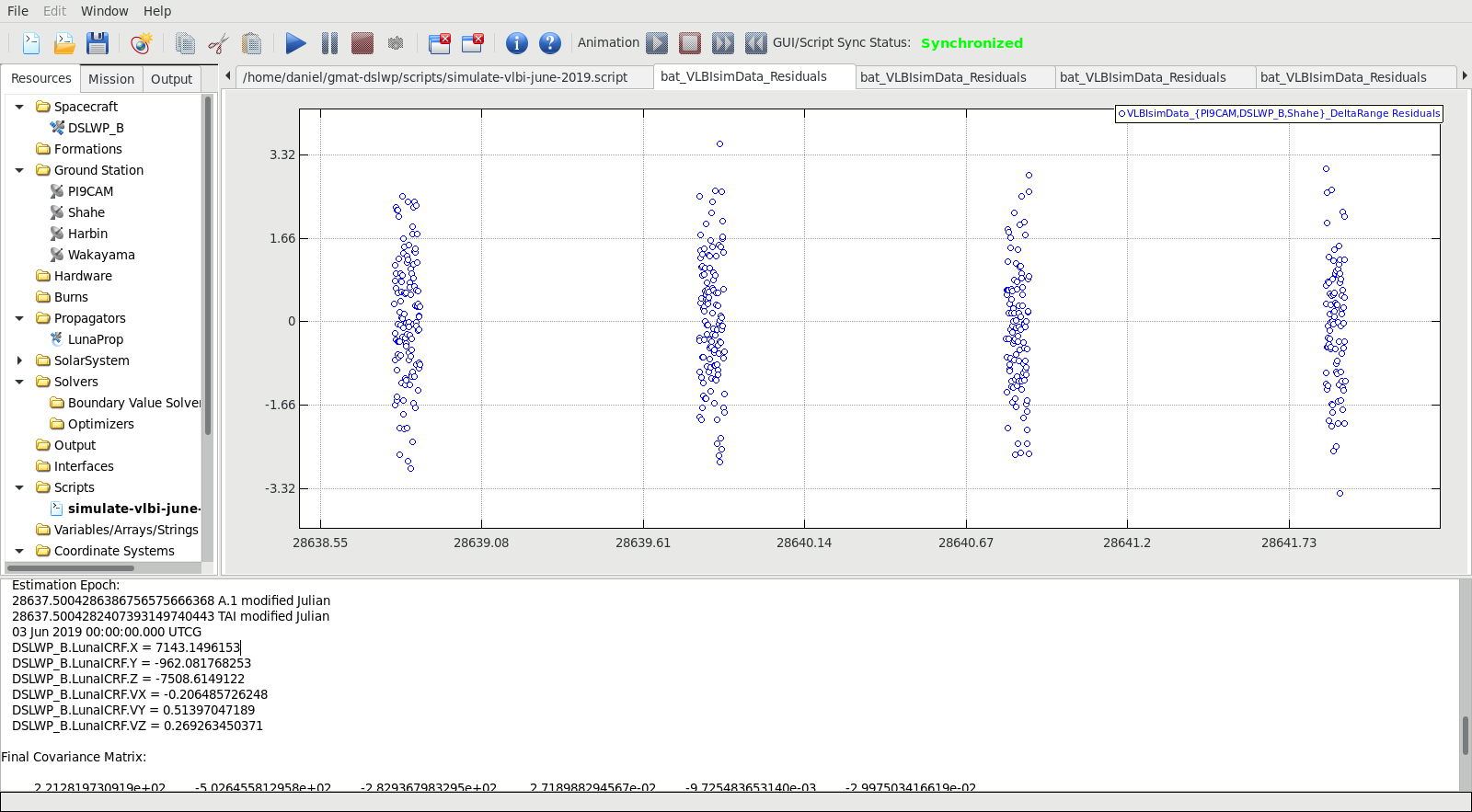
The figure below shows the results of running estimation with a batch filter using the simulated observations. The delta-range residuals of one of the baselines can be seen in the plot.
Mathematical definition for delta-range rate
In my previous post I gave the precise definition for delta-range, taking appropriate care about the light-time corrections. The definition for delta-range rate is easier, as it is the incremental quotient of delta-range. If \(d(t)\) denotes the delta-range at observation time \(t\) (recall that the observation time is defined as the instant that the signal arrives to the reference station), and \(T\) denotes the “Doppler count interval”, then the delta-range rate at observation time \(t\) is\[\frac{d(t) – d(t-T)}{T}.\]
Delta-range derivative computation
The derivative computation for the DeltaRangeAdapter is based on the computation done for the TDRSDopplerAdapter. Since a delta-range is the difference of two ranges, its derivative is just the difference of their derivatives. However, there is an important peculiarity regarding the state transformation matrices and how GMAT computes derivatives with respect to velocity.
Let’s say we have a range between a spacecraft and a groundstation and we want to compute the derivative with respect to the position of the spacecraft. Then this is done basically by projecting onto the line of sight the unit vector corresponding to the direction in which the derivative is taken. However, if we want to compute the derivative with respect to velocity, then it matters if the range observation timestamp is the transmission time by the spacecraft or the reception time by the groundstation.
If the timestamp is the transmission time, then the derivative is zero, as nothing changes about the range measurement with respect to the spacecraft velocity. If however the timestamp is the reception time, then the position of the spacecraft at transmission time depends on the spacecraft’s velocity, and so the derivative is not zero in general.
In a delta-range calculation the situation is a bit tricky. For the reference leg, we timestamp at reception time, so everything goes as expected. However, for the other leg the timestamp is taken at transmission time, and taken to coincide with the transmission time for the reference leg. If we don’t do anything special, the derivative with respect to velocity of the other leg will be computed incorrectly.
The trick I have done is to copy over the state transformation matrix from the reference leg into the other leg. This gives the correct calculation, because it includes the light-time of the reference leg, which is also what should be used when computing the derivative of the other leg with respect to velocity.
I have validated that with this trick the derivative calculation is correct by doing a detailed simulation as in my previous post, where I use debug macros to print out intermediate values. By changing slightly the state vector of the spacecraft (both for position and for velocity) I can check if the changes in the delta-range match what predicted by the derivatives.
Delta-range rate computation
Delta-range rate is computed following the approach of TDRSDopplerAdapter. As shown in the mathematical definition, there are two “paths” subtracted: the end-path, which is timestamped at the observation time \(t\), and the start-path, which is time timestamped at \(t-T\). The way this is done so that derivatives are correctly computed in GMAT is to timestamp both paths at \(t\) and include the \(-T\) in the start-path as a receiver delay. This is done by using the method SetCountInterval() to set the correct value for \(T\).
For the delta-range rate computation, SetCountInterval() only needs to be called for the reference leg of the S-path, since the other leg has its timestamp already affected by the receiver delay applied to the reference leg.
Using debug simulations which print out many intermediate calculations I have checked that the calculations for delta-range rate and its derivatives are correct.
Further work
Even though this project is quite usable as it stands now, I have still some things to do. First, even though I announced in my previous post that I would have per baseline error models, this isn’t working yet. The problem is that groundstations don’t accept several error models of the same type assigned to them (and a groundstation would have an error model per baseline it participates in). This behaviour can be changed, but it is implemented in the StationPlugin, so I will have to go and build and modify that plugin as well.
Then, I marked myself a few TODOs and notes as I wrote the code. None of these are probably very important, since the code seems to be working anyway, but it would be good to review them.
Finally, the code should be tested with some of the real VLBI observations we have for DSLWP-B. This will involve reviewing the correlation and measurement calculation code to make sure it complies with the mathematical definitions of delta-range and delta-range rate given here and in the previous post. Perhaps something will need to be adapted, since I wasn’t as careful with the timing of events when I implemented the correlation code (in particular, regarding the lack of symmetry between the reference and other stations).