One of the things I’ve always wanted to do since Es’hail 2 was launched is to perform two-way ranging by transmitting a signal through the Amateur transponder and measuring the round trip time. Stefan Biereigel DK3SB first did this about a year ago. His ranging implementation uses a waveform with a chip rate of only 10kHz, as it is thought for Amateur transponders having bandwidths of a few tens of kHz. With this relatively slow chiprate, he achieved a ranging resolution of approximately 1km.
The QO-100 WB transponder allows much wider signals that can be used to achieve a ranging resolution of one metre or less. This weekend I have been doing my first experiments about ranging through the QO-100 WB transponder.
Overall summary
Since this post is rather long, I will start with a brief summary. I have designed a waveform that is based on the Galileo E1C Open Service pilot signal but with a chip rate four times slower with the goal of using it to perform two-way ranging of Es’hail 2 by transmitting this waveform through one of the 1Mbaud DVB-S2 channels in the WB transponder.
Synchronization of the RX and TX streams of the LimeSDR mini that I’m using for this experiment has been somewhat tricky, but seems more or less solved now.
I have made Python code from the scratch to acquire and track this ranging signal, and to compute round trip time measurements. Over the air tests by doing transmissions of a few minutes through the transponder show that the system is working well and produces a ranging result that matches the GEO location of Es’hail 2. Ignoring systematic errors, the precision of this ranging method is on the order of one meter or better.
The material for this post can be found in this repository.
Waveform design
I have decided to use a ranging waveform that is based on the Galileo E1C Open Service pilot signal. The reasons for this design choice are the following. First, it is something I know very well from my dayjob; second, with this I want to try to get more Amateur radio operators interested into GNSS in general; third, maybe some software tools intended for Galileo can be repurposed to use them with this waveform; and finally, the spectrum of this signal has two sidelobes, so this prevents annoying other operators that may mistake the ranging signal for a DVB-S2 signal (which represents almost all the traffic through the WB transponder) and fruitlessly try to decode it as such.
The design constraint is that the waveform must fit into a 1Mbaud DVB-S2 channel. There are two reasons for this. First, while a wider signal might be used over the WB transponder for short experiments (there are approximately 7.5MHz of the transponder which are not occupied by the DVB-S2 beacon), such an atypical use would need to be fairly limited in time, and coordinated with the rest of the transponder users. By designing a waveform that acts as a 1Mbaud DVB-S2 signal from a spectrum management point of view, it is easier to share the transponder with all the other users, by following the usual operating practices. Second, the Beaglebone black ARM computer I have in my QO-100 groundstation is limited to around 2Msps full-duplex with the LimeSDR mini. If I want to use a wider signal, I would have to upgrade the hardware.
The Galileo E1C signal is a BOC signal with a chip rate of 1.023Mchip/s (for those that know the details, the E1C signal is actually a CBOC signal, but here I’ll pretend it’s just BOC). BOC is a terminology used in GNSS to denote a BPSK signal in which the chips are Manchester encoded. This produces two sidelobes in the spectrum. As the ranging performance of a waveform is determined by its RMS bandwidth (the standard deviation of its power spectral density), the sidelobes of a BOC signal serve to send energy away from the centre of the modulation, increasing the RMS bandwidth and so the ranging performance. For this reason, BOC signals are used in many modern GNSS waveforms, such as the Galileo E1 signals, the GPS L1C signal, the Beidou B1C signal, and the QZSS L1C signal.
The chip rate of 1.023Mchip/s is too high to fit into a 1Mbaud DVB-S2 channel. In fact, the bandwidth of the main lobes of the BOC modulation is 4.092MHz. However, we can divide the chip rate by four and use a chip rate of 255.75kHz, so that the bandwidth of the main lobes becomes 1.023MHz.
GNSS signals often use unfiltered pulse shapes, in order to improve the ranging performance. Therefore, their total bandwidth is very large, since they have many sidelobes. To obtain a ranging waveform for the QO-100 WB transponder, we need to filter out the sidelobes. In the transponder bandplan, 1Mbaud channels have allocated 1.5MHz of spectrum, in order to leave some guard band for adjacent DVB-S2 signals with an excess bandwidth of 0.35, which have a bandwidth of 1.35MHz. For the design of the ranging waveform, we take this bandwidth as a guide and filter the waveform to a bandwidth of 1.35MHz.
The E1C signal uses a PRN of 4092 chips and a secondary code of 25 symbols. This means that each of the repetitions of the PRN is multiplied by one of the symbols of the secondary code, so the whole chip sequence repeats after 102300 chips. The PRNs are memory codes, meaning that they are not generated algorithmically. They have been found by a search process that minimizes autocorrelation sidelobes and cross-correlation against other PRNs in the set.
The secondary code of the E1C signal repeats every 100ms. Since we are using one fourth of the chip rate, our ranging waveform repeats every 400ms. Since round trip time to GEO is on the order of 260ms, our waveform can perform unambiguous round trip time measurements.
For using a single ranging waveform, an LFSR would be ideal as the PRN, since it has minimal autocorrelation sidelobes. However, I think it is interesting to allow for the possibility of having several simultaneous ranging signals transmitted by different stations, so I have decided to use one of the PRNs for Galileo E1C.
Since the ranging waveform uses different a carrier frequencies and chip rate in comparison to the real Galileo E1C signal, interference to Galileo equipment is very unlikely. But even so, I have decided to use PRN 42, which is not to be used by any of the real Galileo satellites. The Galileo signals have a set of PRNs numbered 1 through 50, but only PRNs 1 through 36 are to be used in the real satellites.
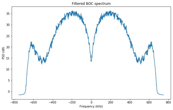
To sum up, the ranging waveform is exactly the same as the Galileo E1C signal for PRN 42, but with a chip rate of 255.75kHz, so everything runs 4 times slower, and filtered to a bandwidth of 1.35MHz. In the Signal generation Jupyter notebook I have included all the details about the generation of the signal. A sample rate of 1.5Msps is used throughout this post. The figure below shows the spectrum of the filtered signal. Note that the filter lets in part of the secondary lobes.
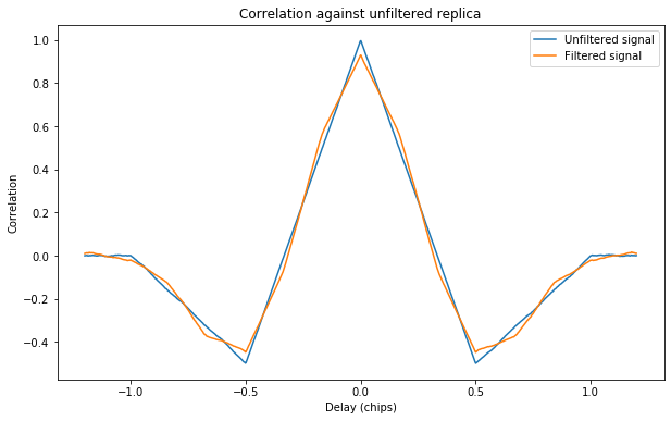
Below we can see the correlation of the filtered waveform against an unfiltered replica, compared to the autocorrelation of the unfiltered waveform. We see that the difference is small, so not much performance is lost by filtering the waveform.
LimeSDR-mini synchronization
A very important thing when using an SDR transceiver for ranging is to be able to synchronize the RX and TX sample streams. Since ultimately we are measuring the delay between the transmitted and received waveforms, we need to know the delay between the sample streams, if any. Most SDRs use the same sample clock for RX and TX, so when the RX and TX are already started, their relative delay will be constant (unless we lose samples).
My idea was to first set the RX channel to the same frequency as the TX channel, in order to receive the transmit waveform through leakage. This can be used to determine the offset between the RX and TX sample streams (which should be an integer number of samples). After recording the TX waveform for a few seconds, we would switch the RX frequency to tune it to the transponder downlink frequency (or rather its IF after downconversion by the LNB) without stopping the sample stream. Then the round trip time through the transponder could be measured. However, this didn’t work as expected. It turns out that changing the RX frequency (for example by calling LMS_SetLOFrequency()) interrupts the sample stream in an unpredictable way.
Rather than trying harder to make this approach work, for instance by finding a lower level way to change the RX frequency, I decided to try to obtain a repeatable RX-TX synchronization behaviour by using hardware timestamps, inspired by the dualRXTX.cpp LimeSuite example. It turns out that every time that you get a buffer of RX samples using LMS_RecvStream(), you can get the hardware timestamp for the first sample in this buffer in an lms_stream_meta_t structure. This hardware timestamp is just a sample counter which is shared between RX and TX. Then, when submitting a buffer of TX samples using LMS_SendStream(), we can use an lms_stream_meta_t to specify the hardware timestamp at which the first sample of this buffer should be transmitted.
So we do the following with this hardware timestamping functionality. We get our first buffer of RX samples and take note of the hardware timestamp. Then we increment this timestamp in 1024*128 samples and send the first TX buffer marked to be transmitted at this future timestamp. The delay of of 1024*128 samples is so that the call to LMS_SendStream() can get through completely before the required time for start of TX arrives. Instead of starting the transmission by the first sample of the ranging waveform, we skip the first 1024*128 samples. Therefore, the effect is as if the transmission of the ranging waveform had started at the same time that the first RX sample was taken. After sending this timestamped TX buffer, we do not use hardware timestamping anymore and proceed normally, getting samples from the RX buffer and sending samples into the TX buffer in order to prevent overruns or underruns.
There is another quirk regarding this synchronization scheme. For some unknown reason, shortly after starting the RX stream, a few RX packets are dropped, as reported by the droppedPackets field in the lms_stream_status_t. This causes a few thousands of samples to be missing from the RX stream, which offsets the TX and RX samples. What I do to get around this problem is to drop to the floor the first 48300 RX samples, so that the droppedPackets happen as part of these ignored samples. After this, I start recording RX samples and bootstrap the RX-TX synchronization as described above.
Even after all this, the RX-TX synchronization is not perfect. By tuning the RX channel to the TX frequency and receiving the TX ranging waveform through leakage, I have determined that the RX and TX streams are still offset by 93 samples. Fortunately, the effect is repeatable almost always (on rare occasions I find an offset of 92 or 94 samples instead). I correct for this offset later by dropping the first 93 RX samples.
The software I use to drive the LimeSDR mini can be found in limesdr_ranging.c. This is still in a rather crude state, but it works. It is based on my limesdr_linrad.c. It reads the TX waveform from a file and keeps looping it, and streams RX samples through the network by using the Linrad protocol. The frames are received and recorded in another PC by using socat as
socat UDP4-RECV:50100,reuseaddr - | pv > /tmp/ranging.int16
Linrad is used to monitor the received signal.
Acquisition and tracking
After the downlink signal has been recorded, the ranging waveform is acquired and tracked. I have made my own implementation of these algorithms, but most likely existing tools for Galileo can be used by lying to them and saying that the sample rate of the recorded signal is 6Msps rather than 1.5Msps (to compensate for the fact that the ranging signal is four times slower than Galileo E1C). For instance, the great GNSS-DSP-tools Python scripts by Peter Monta can be used.
The acquisition is rather easy, since the signal is much stronger than the typical GNSS signal. Therefore, an FFT-based correlation with a single PRN repetition (16ms coherent integration time) is more than enough to have good acquisition SNR. Moreover, the range of Dopplers that needs to be swept is small (see this post, for instance, for the study of Es’hail 2 Doppler).
The acquisition produces frequency and delay estimates that are used to start the tracking. Tracking is done in the same way as for GNSS signals. We start by performing tracking for the first 100 symbols using a Costas PLL, in order to find the correct secondary code phase. Then the tracking is restarted from the beginning of the recording and we use a pure (non-Costas) PLL and secondary code wipeoff. A coherent integration period of 16ms is used for both the PLL and the DLL, and the DLL uses a coherent discriminator with an E-L spacing of 0.1 chips. I haven’t adjusted the loops yet. I have simply eyeballed some coefficients by trial and error, without taking care for critical damping, etc.
The code for acquisition and tracking can be seen in the tracking.py Python file.
Over the air testing
After doing several loopback tests receiving my own signal, I passed to over the air testing through the QO-100 WB transponder. The first over the air test was done at around 20:00 UTC on 2020-06-13. The WebSDR screen during the test can be seen below.

A transmit frequency of 2403.75MHz was used, thus occupying the first 1Mbaud DVB-S2 channel. Care was taken not to interfere with other stations by selecting a channel that was free at that moment. The transmission lasted only a few minutes, which is more than enough to measure round trip time and observe its drift with time.
For the test I used my QO-100 groundstation, which currently has a 24dBi linearly polarized grid parabola as transmit antenna, a 100W PA (though I wasn’t driving the PA to saturation and don’t know exactly how much power I was using) and a 1.2m offset dish as receive antenna.
Unfortunately, for this test I still hadn’t detected the problem of sample stream interruption when the RX frequency was changed, so the round trip time I computed was all wrong. Therefore, I made additional over the air tests around noon on 2020-06-14.
To identify my transmissions, as mandated by the Amateur radio regulations I’m using a very crude but perhaps effective method. I’m keying on and off the transmission of the ranging waveform by using my callsign in Morse code. I do this when I’m not recording the receive signal for ranging measurement, as for this I need a steady signal.
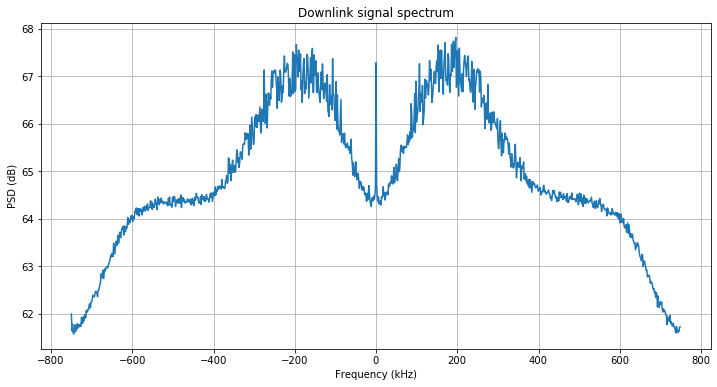
The figure below shows the spectrum of the downlink signal for a test done around 11:56 UTC on 2020-06-14. The (S+N)/N is approximately 2.5dB. The peak in the center is the TX DC spike (TX LO leakage plus ADC voltage offsets). For RX there is no DC spike, since I’m using the LMS7200M NCO to place the DC spike outside the passband.
The correlation IQs obtained by tracking the downlink signal with the Costas PLL can be seen below. The repeating secondary code is clearly visible. The keen reader might already get an estimate for the round trip time from this figure by observing in which phase the secondary code appears.
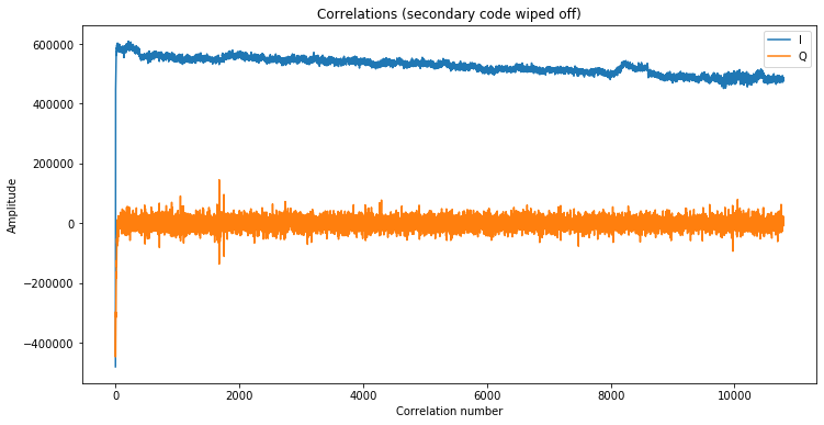
After the phase of the secondary code has been determined, tracking with a pure PLL and secondary code wipeoff is done. The IQs are shown below. The slight droop in the in-phase component is probably due to changes in the gain of my PA as it gets hot.
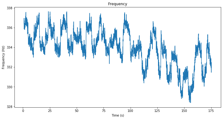
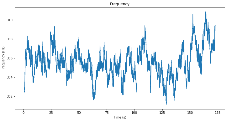
The measurements generated by the tracking are saved to an npz file and then analysed in this Jupyter notebook. The figure below shows the tracking frequency. It is not zero for a number of factors: Doppler (which only accounts for approximately 30Hz), transponder LO error (which in my studies of the NB transponder doesn’t seem that large), and offsets in my system such as fractional-N PLL errors, LMS7200M NCO quantization error, etc.
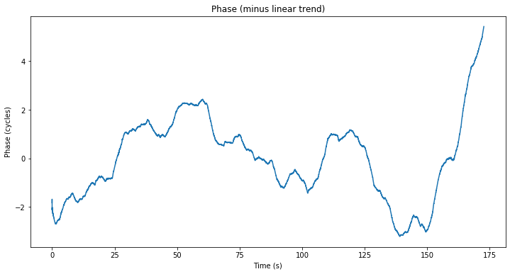
Next we plot the carrier phase, from which we’ve removed its linear trend in order to be able to see something. Since the transponder LO affects the downlink signal phase, using the phase observations is not very useful unless we had two stations transmitting simultaneously and we subtracted the observations corresponding to each of them.

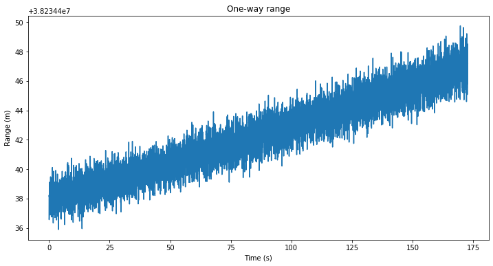
Finally, we show the one-way range, which is defined as the round trip time divided by two and multiplied by the speed of light. We do not include the first measurements, as the round trip time starts off by its value coming from acquisition and then moves quickly several tens of metres to converge to the appropriate value.
Note the way the plot is done in Matplotlib with an offset shown in the corner upper left corner. The one-way range is actually around 38234322.0 metres. The units of the scale are metres, so the code tracking noise is on the order of one metre RMS without even having to tune the DLL loop carefully.
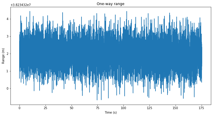
It is interesting that the one-way range is almost constant throughout the 3 minute recording. This is because the time of closest approach from Es’hail 2 to my station is around 12:00 UTC. When this recording was done, the Doppler was near zero and the range changed very slowly.
To check this effect, I made a second test roughly one hour later, at 12:48UTC. The correlations for the second test can be seen below. They show a similar behaviour to the first test.
Below we show the tracking frequency. It has decreased 27Hz in comparison to the first test. This can’t be caused by a change in Doppler, as it doesn’t change that much in one hour. I think that I may have used a different 1Mbaud DVB-S2 channel for this test, since the channel where I did the first test was now in use. If this is true, then this can explain the difference, since changing the TX and RX frequencies involves a new set of fractional-N PLL errors.
The phase observations don’t really show much, as it was the case during the first test.
The one-way range now shows an average value of 38234442.3 metres, which is 120.3 metres more than in the first test. Since there was a difference of approximately 52 minutes between the tests, this gives an average rate of 38.6mm/s. During this test we see a rate of change of one-way range of approximately 52.3mm/s. This matches the spacecraft exiting its point of closest approach to my station and starting to move away. Near the point of closest approach, the range evolution with respect to time is approximately a parabola.
Systematic errors
In these ranging measurements there are the following systematic errors. The most important error comes from the fact that the round trip time measurement is ultimately determined by the sample rate of the SDR. My whole groundstation is locked to a 10MHz GPSDO, but even so the sample rate is not exactly 1.5MHz because of the fractional-N PLL errors involved in the synthesis of the sample clock: a 27MHz DF9NP PLL, and the LMS7002M. Fractional-N PLLs multiply their input frequency by a fraction that (usually) has a large numerator and denominator, and which is quite close to (but not exactly) the nominal multiplication ratio. For precise results, the actual PLL multiplication ratio needs to be determined. The errors can be on the order of ppm’s, which when related to the range measurement can give an error of a few hundreds of meters.
Next, there is the delay of the WB transponder. This is unknown. Measuring the transponder delay in orbit is not easy, since the orbit of the satellite and all other sources of error need to be computed to better precision than the transponder delay. In a similar manner, there are the delays associated with my groundstation hardware and the fact that my transmit and receive antennas are a few metres apart.
There are also atmospheric errors. The ionospheric delay plays a small role at the 2.4GHz uplink, with a contribution of 7cm per TECU, and an insignificant role at the 10.5GHz downlink, with a contribution of 3.6mm per TECU. The tropospheric delay is thus more important. Since the troposphere is non-dispersive, the effect doesn’t depend on the frequency, and usually amounts to a few meters.
While it is not really an error, but rather a particularity of this measurement, one must take into account the fact that light doesn’t travel in straight lines in ECEF coordinates, which are the natural coordinates for this GEO ranging measurement. Thus, the Earth rotation is usually introduced as a correction to the measurement. See this post for details.
Finally, there are relativistic errors, but I think they are very small and can be ignored.