The first Amateur VLBI experiment with DSLWP-B was performed on 2018-06-10. In that experiment, the 250baud GMSK beacons at 435.4MHz and 436.4MHz were recorded in the 25m PI9CAM radiotelescope in Dwingeloo, The Netherlands, and a 12m repurposed Inmarsat C-band dish in Shahe, Beijing. These synchronized recordings were processed later to obtain delta-range and delta-velocity measurements. Due to the low baudrate, the noise of the delta-range measurements was quite high, on the order of 20km. Since the beacons were short transmissions of 15 seconds, making accumulated phase measurements was not possible.
Another Amateur VLBI experiment was performed on 2018-11-21. The novelty of this experiment was that 500baud GMSK SSDV transmissions were made on 436.4MHz. These long transmissions, lasting around 30 minutes each, allow us to make accumulated phase measurements. Also, the higher baudrate reduces the noise in the delta-range measurements. Another novelty was that a third station, the Harbin Institute of Technology Amateur Radio Club BY2HIT groundstation also joined the experiments, so observations from three stations are available.
This post is an account of the results I have obtained processing the observations from 2018-11-21.
Observation correlation
The observations of the three groundstations can be downloaded from the file repository of CAMRAS (search for 2018-11-21). The format of these files is the GNU Radio metadata format, with 32 bit float IQ samples and 40ksps. The first step in processing these files is to use convert_metadata_file.py to convert the files to complex64 IQ files, removing the metadata. This makes it easier to process the files with NumPy later.
The next step is to take note of the timestamp corresponding to the start of each of the recordings. This is stored in the file metadata and can be read by using
gr_read_file_metadata $file | grep Seconds | head -n 1
The correlate_recordings.py script is the main piece of the pipeline for processing the observations. It reuses many signal processing blocks from my Moonbounce processing pipeline. The script runs on each baseline (i.e., on each pair of recordings) and performs the following tasks:
- Alignment of the recordings according to the timestamps
- Calculation of expected Doppler using GMAT
- Correction of expected Doppler on each observation
- Lowpass filtering of each observation
- Correlation in time and frequency using FFTs
The correlation algorithm is very similar to the one used in the first Amateur VLBI experiment, but the FFT size is \(2^{17}\) samples, or 3.2786s, so as to give a good balance between SNR and update rate of measurements.
All the results are saved to either NetCDF4 files using xarray or NPY files for later analysis.
The script needs to take into account the frequency offset of the transmitter on-board DSLWP-B, so as to correct this offset to bring the signal to baseband before lowpass filtering the observation. This offset was determined using the Moonbounce processing scripts to be -250Hz for the 436.4MHz transmitter. The 435.4MHz recordings have not been processed yet, since they are not so interesting, as they only contain short GMSK beacons.
Since the Python script takes a lot of parameters, the Bash script run.sh is used to run the script with the correct parameters on each of the recordings. The output files can be found here.
Observation postprocessing
The output files of the correlation script are loaded and processed in a Jupyter notebook to compute and evaluate the VLBI measurements. Besides the output files, two additional values are needed in this notebook. These values are printed out by the correlation script and stored in the log.
The first of them is the timestamp associated to the first sample in the correlation. This is computed by the correlation script because it can remove samples from the start and end of each observation in the baseline in order to line them up in time. The second is the residual clock offset. The correlation script tries to line up the two observations perfectly according to their respective timestamps, but it does so by shifting an integer number of samples. Therefore, a clock offset smaller than a sample period might remain after this step. This clock offset must be applied later in order to correct the measurements.
The postprocessing of the correlation outputs produces two types of measurements: delta-range measurements using time difference of arrival, and accumulated phase difference measurements. The accumulated phase differences also measure the delta-range, but they have an unknown offset, and are subject to other additional problems which I will explain later. However, phase measurements are much less noisy than the delta-range measurements, as they use the carrier phase, which is 436.4MHz, a much higher frequency than the 500baud modulation rate.
The accumulated phase differences can be differentiated in time to obtain delta-velocity measurements using the Doppler difference, as it was done in the first experiment. These are very accurate, since they are also derived from the carrier phase.
Measurements filtering
As it has been the case in previous Amateur VLBI experiments using low baudrate signals not intended for ranging, such as the first DSLWP experiment and the LilacSat-2 experiment, there is a huge gap between the precision of the measurements derived from time difference of arrival, such as the delta-range, and the phase difference, such as the delta-velocity. The error of the delta-range measurements is on the order of 10km, while the error in the delta-velocity measurements is on the order of 0.1m/s.
To try to bridge this gap, it is possible to use the delta-velocity measurements to smooth out or filter the delta-range measurements. Here I have tested two different smoothing algorithms to evaluate their performance.
The first of them is usually called the Hatch filter in the GNSS literature. If \(r_k\) and \(v_k\) are the delta-range and delta-velocity measurements respectively, we compute filtered delta-range measurements \(y_k\) as\[y_k = \alpha r_k + (1-\alpha) (y_{k-1} + v_k),\]where \(\alpha > 0\) is a small parameter. Thus, we see that the Hatch filter is just a weighted average between the current non-smoothed delta-range and the previous smoothed delta-range propagated using the delta-velocity.
For very small values of \(\alpha\) the filter gives out a very smooth output, but it might drift from the true value, since errors in the propagation using the velocity accumulate. For larger values of \(\alpha\) the output is not so smooth but it follows the measurements \(r_k\) more closely.
The second method I’ve used is the Kalman filter. The model on which this filter is based considers a state \(x_k\) which evolves linearly with some stochastic perturbations as\[x_{k+1} = F x_k + n_k,\]where \(n_k\) is known as the process noise and is Gaussian with covariance \(Q\). The state is observed linearly, with some measurement noise, to produce observations\[z_k = Hx_k + m_k,\]where the measurement noise \(m_k\) is Gaussian with covariance \(R_k\).
The Kalman filter is an optimal estimator for the state \(x_k\) and the state error covariance \(P_k\) given a series of measurements \(z_k\) and their error covariances \(R_k\).
In our case, we consider a really simple model where the state is \(x_k = (r_k, v_k)^T\), the measurement matrix is \(H = I_{2\times 2}\), the state evolution is\[F = \begin{pmatrix}1 & 1\\ 0 & 1\end{pmatrix},\] and \(Q\) and \(R_k\) are diagonal matrices.
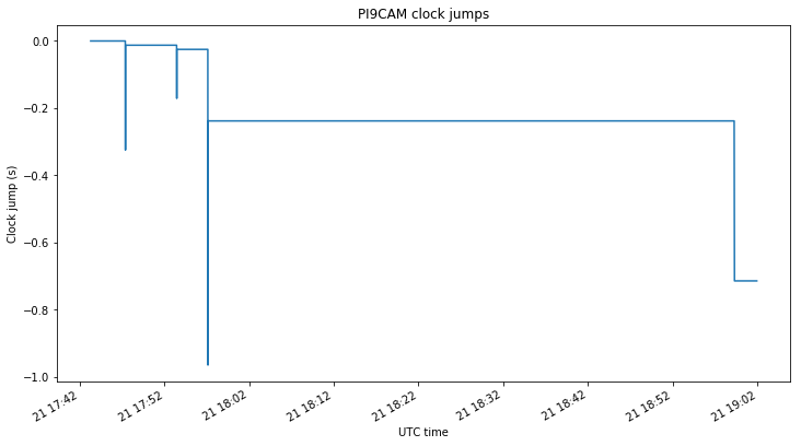
Correction of clock jumps
The PI9CAM recordings have clock jumps, probably caused by lost samples while the recording was made. However, since the GNU Radio metadata file format saves timestamps periodically, it is easy to compute and correct these clock jumps. The figure below shows the jumps in the clock of the PI9CAM recording. These are corrected in the correlation postprocessing, by adding the clock offset to the computed delta-range.
Evaluation of the measurements
After obtaining the measurements, the Jupyter notebook is used to plot and evaluate them. The figure below shows the amplitude of each of the correlations.

We can see that each of the baselines has a different time span, since PI9CAM joined the experiment late and Harbin finished earlier. The short spikes correspond to GMSK telemetry beacons, while the long periods when the signal is transmitting correspond to SSDV image downlinks. We see that the SNR on the PI9CAM-Shahe and PI9CAM-Harbin baselines is an excellent 40dB, while the SNR on the Shahe-Harbin baseline is only 20dB. This gives lower quality measurements, but the measurements for the Shahe-Harbin baseline can also be obtained by subtracting the PI9CAM-Harbin and PICAM-Shahe baselines, thus obtaining lower noise measurements than if using this baseline directly.
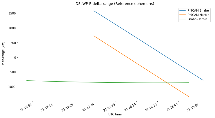
According to the GMAT ephemeris, the delta-range measurements on each of the three baselines should evolve as shown in the figure below.
The three figures below show, for each baseline, the offset between the delta-range VLBI measurements and the GMAT reference ephemeris. Unfiltered, Hatch filtered and Kalman filtered measurements are compared.
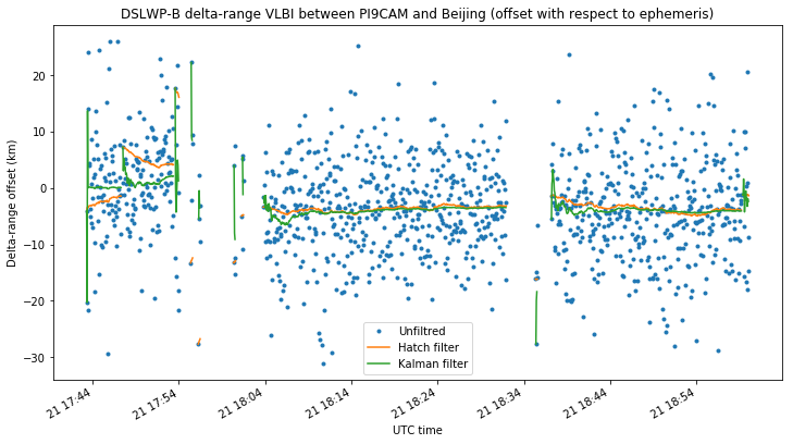
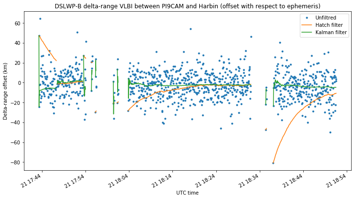
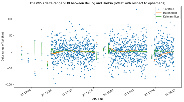
The jumps in the filtered measurements during the first SSDV transmission on the PI9CAM baselines are caused by one of the PI9CAM clock jumps. The filters are reset at the clock jump due to unavailability of measurements during the clock jump.
We see that the delta-range noise in the unfiltered measurements for the PI9CAM baselines is around 10-20km. On the Shahe-Harbin baseline it is on the order of 50km, due to the much lower SNR. The noise of the filtered measurements is much lower, so we plot them below without the unfiltered measurements to examine them in more detail. The three plots use the same vertical axis to ease comparisons.
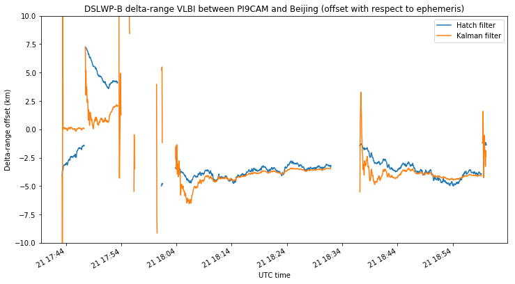

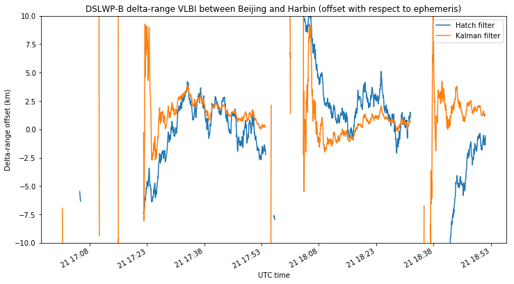
These plots illustrate the main difference between the simple Hatch filter and the more complex Kalman filter. The Hatch filter doesn’t have memory, and performs in the same manner during the course of an observation. This makes adjusting the parameter \(\alpha\) tricky. Too small and the filter will take a lot of time to converge to the correct value, as it happens in some of the plots above if the filter was started with a delta-range measurement with a large error. Too large and the filter will be very noisy.
On the other hand, the Kalman filter propagates the covariance of the state error \(P_k\) and uses it to vary the smoothing as time progresses. In the beginning of each transmission, the filter doesn’t have a good estimate of the state \(x_k\), so it tries to move quickly to converge to a good estimate, giving a noisier output. As the transmission goes on, the filter gains confidence in its estimate of the state \(x_k\), reducing the noise in its output at the expense of responding more slowly to unexpected jumps in the state.
We see that, for the PI9CAM baselines, the noise of the Kalman filter is very small in comparison with the unfiltered delta-range measurements, perhaps on the order of 100m. On the other hand, the Shahe-Harbin baseline gives a noise of around 1km, owing to the much lower SNR.
There seems to be a bias of around -5km, -2.5km and 2.5km in the delta-range measurements of each baseline respectively. This is probably caused by errors in the reference ephemeris used in GMAT. However, it is convenient to note that in comparing the VLBI measurements with the GMAT ephemeris we are using a simple model that ignores the finite propagation speed of light. It is assumed that the delta-range at time \(t\) is given by\[\|s(t) – g_1(t)\| – \|s(t) – g_2(t)\|,\]where \(s\), \(g_1\) and \(g_2\) denote the position of the satellite, first groundstation and second groundstation respectively. However, in reality, the delta-range at time \(t\) is given by the more complicated formula\[\|s(t-\tau_1(t)) – g_1(t)\| – \|s(t-\tau_2(t)) – g_2(t)\|,\]where the propagation delays \(\tau_j\) satisfy\[c\tau_j(t) = \|s(t-\tau_j(t)) – g_j(t)\|.\]
Phase measurements
As I have already mentioned, phase difference measurements give very good precision, as they use the relatively high carrier frequency to measure delay, instead of using the low baudrate modulation. However, they have several associated problems that need to be treated carefully.
First of all, phase difference measurements have an ambiguity or offset. In the ideal case when the local oscillators of the two stations participating in the baseline are perfectly synchronized, this offset is an integer number of cycles which is caused by the fact that the phase can only be measured modulo one cycle. Performing accumulated phase measurements, i.e., relating a phase measurement with the measurement of the previous epoch allows us to have a common offset for the complete sequence of measurements, instead of having a different and unrelated offset per measurement. If one wants to give physical meaning (as delta-ranges) to the phase difference measurements, this unknown integer number of cycles needs to be determined.
However, usually the local oscillators in the groundstations are synthesized using PLLs, and these can lock to a different phase offset every time they are started. In practice, this means that the local oscillators of the two groundstations participating in the baseline are not synchronized, but rather have an unknown and fixed offset. The consequence is that the offset for the accumulated phase measurements is no longer an integer, but any value. Therefore, it cannot be determined exactly, but only approximated.
The usual procedures for determining the phase offset involve filtering delta-range measurements based on the modulation, which are unbiased. If the noise of these measurements can be reduced to less than one wavelength, then an integer phase offset can be determined exactly. In the case of DSLWP-B, the difference in precision of the modulation-based and phase-based measurements is so large that it is probably impossible to use this kind of procedures.
Another problem regarding phase measurements is errors in the frequency of the transmitter. Indeed, if the nominal frequency of the transmitter is \(f\), an error of \(\delta f\) will cause an error in the determination of velocity of\[\delta v = v \frac{\delta f}{f}.\]Integrating this error over a time interval \(0 \leq t \leq T\) produces an error in delta-range of\[\delta r = (r(T)-r(0))\frac{\delta f}{f}.\]
In the case of DSLWP-B, the change in delta-range over the course of an observation is on the order of \(10^6\)m. Therefore, a frequency error of 1ppm (which is a good assumption for the DSLWP-B TCXO) produces an accumulated error of 1m at the end of the observation. This is small in comparison with other sources of error, so this kind of errors can be ignored.
In any case, the performance of the phase difference measurements can be evaluated by plotting the diference between the delta-range obtained from these measurements and the reference ephemeris. The average needs to be subtracted, so as to remove the unknown offset in the accumulated phase. This is shown in the figures below.
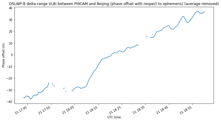
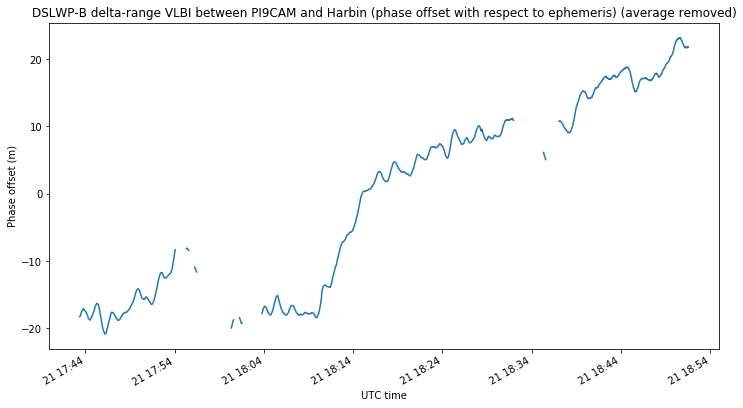

We can see that the noise of the phase measurements is sub-metric, as is to be expected. An error of several tens of metres accumulates with time. This is most likely due to small errors in the reference ephemeris.
It is also noticeable that the phase measurements show some kind of wavy pattern. This is best seen in the delta-velocity measurements, which are the time derivative of the plots shown above.

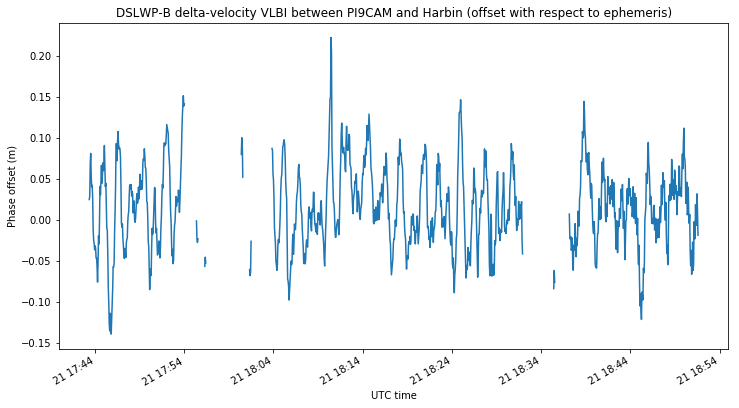
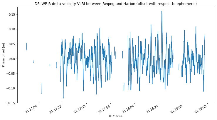
The cause of this oscillating error is not known. It might even be caused by errors in the frequency references of the groundstations. Even though each groundstation uses a GPSDO, the frequency reference can have some small errors, since a GPSDO works by estimating the phase error of a voltage-controlled oscillator and steering it to phase-lock it to GPS time. The error seen in the figures above corresponds to a reference frequency error of 0.2ppb, which is perfectly compatible with the steering error of a GPSDO.
Conclusions
We have seen that the error in delta-range measurements using time of arrival measurements is large, on the order of 10km, due to the low baudrate modulation used for the VLBI experiment. On the other hand, measurements derived from observing the carrier phase have an error of sub-metric level. It doesn’t seem possible to bridge this gap of 4 orders of magnitude and use unbiased delta-range measurements to remove the inherent biases in phase-based observations.
The use of simultaneous carrier phase observations on 435.4MHz and 436.4MHz would provide a 1MHz signal to obtain estimations having an error of metric or decametric level and ambiguity of an integer number of 300m wavelengths. Therefore, it might be possible to use a tiered approach where unbiased modulation-based observations are used to compute the unknown integer number of cycles for the 1MHz signal, and the relatively low noise of the (now bias free) 1MHz signal is used to obtain unbiased carrier phase based measures. This would require simultaneous long transmissions in both bands, but this hasn’t been performed so far due to concerns of overheating in the transmitter.
There are some unknown biases present between the observations and the reference ephemeris. While an error in the ephemeris can explain these completely, instrumental biases or other biases in the signal processing chain shouldn’t be ruled out completely. These Amateur VLBI groundstations haven’t been commissioned by performing calibration observations, with sources such as a satellite for which precise ephemeris are available. The use of a more complex model for the interpretation of delta-ranges, including the finite propagation speed of light effects would also be a useful exercise.
Finally, the ultimate goal of these observations is to perform precise orbit determination with them. No such attempts have been made yet. Trying to fit an orbital state vector to the observations would serve as additional validation of the observations, ruling out possible errors in the published ephemeris. However, it is convenient to note that the observations analyzed in this post last only a 2 hour activation period of DSLWP-B. To perform accurate orbit determination, observations need to be made at well spaced points along the orbit. The orbital period of DSLWP-B is around 20 hours. Therefore, well spaced activations and observations on the same day or on nearby days should be planned to perform this task. This also makes observation planning tricky due to the requirement of a common window on the longer Europe-China baselines.
4 comments