In March this year I spoke about the Amateur VLBI with LilacSat-2 experiment. This experiment consisted of a GPS-synchronized recording of LilacSat-2 at groundstations in Harbin and Chongqing, China, which are 2500km apart. The experiment was a preparation for the Amateur VLBI project with the DSLWP lunar orbiting satellites, and I contributed with some signal processing techniques for VLBI.
As you may know, the DSLWP-B satellite is now orbiting the Moon since May 25 and the first Amateur VLBI session was performed last Sunday. The groundstations at Shahe in Beijing, China, and Dwingeloo in the Netherlands performed a GPS-synchronized recording of the 70cm signals from DSLWP-B from 04:20 to 5:40 UTC on 2018-06-10. I have adapted my VLBI correlation algorithms and processed these recordings. Here are my first results.
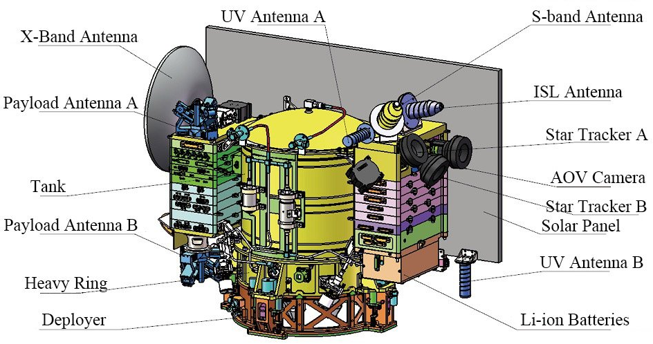
The baseline for these VLBI recordings (i.e., the distance between the groundstations) is roughly 7250km. The signals transmitted by DSLWP-B are 250bps GMSK using an \(r=1/2\) turbo code. Two transmit frequencies are used: 435.4MHz and 436.4MHz. Each transmit frequency uses a different antenna. The antenna marked below as UV Antenna A is used for 435.4MHz, while the UV Antenna B is used for 436.4MHz.
The transmissions are done in packets. A packet lasts about 15 seconds and is transmitted roughly every 5 minutes. Packets are transmitted simultaneously in both frequencies, but the data transmitted in each of the frequencies is different.
The format of the recordings is as follows. Each recording is 20 seconds long (or 19 seconds in some cases) and contains a single packet. It is formed by two files, one for 435.4MHz and the other for 436.4MHz. Each of these files is an IQ file at 40ksps centred at 435.4MHz or 436.4MHz. The format of the files is the GNURadio metadata format. The file metadata can be read with gr_read_file_metadata and contains the UTC timestamps for the IQ stream. These timestamps are needed to synchronize the recordings made at both groundstations, since their start times can be off by a fraction of a second.
The recordings made at Dwingeloo can be downloaded from the CAMRAS data repostiory, while the recordings made at Shahe can be downloaded here.
The correlation algorithm I’m using works as follows. The input of the algorithm is a pair of recordings for the same frequency and time, one at each groundstation. First, ephemeris data computed using GMAT is used to get the approximate Doppler at each of the groundstations. This approximated Doppler is corrected by subtracting 200Hz (since it seems that the DSLWP-B transmitter is not exactly on frequency) and then this estimate is used to translate in frequency each of the recordings to bring the signals to baseband. The signals are then lowpass filtered to a cut-off frequency of 500Hz by a FIR filter with 512 taps. These two signals are correlated in frequency and time using the following method.
Let us denote by \(x_1\) and \(x_2\) each of the signals, by \(\mathcal{F}\) the Fourier transform operator and by \(S\) the operator defined by a circular shift \((Sx)(j) = x(j-1)\) (where indices are understood modulo the length of the signal). Then we compute\[y_n = \mathcal{F}^{-1}(\mathcal{F}x_1\cdot\overline{S^{n}\mathcal{F}x_2}),\qquad -N \leq n \leq N,\]where \(N\) sets the range of frequencies to search for correlation. We search for the \(j\) and \(n\) that maximize \(|y_n(j)|\). These \(j\) and \(n\) give respectively the time offset (in samples) and frequency offset (in Fourier bins) between both signals.
Note that the length of the Fourier transforms is the whole signal. This means that the signal is integrated coherently for its whole duration. While this may seem problematic, I have checked that the coherence of the received signal is quite good and most of the correlation is concentrated in a single Fourier bin, so it is possible to integrate coherently the whole signal.
This also gives very good resolution (0.05Hz). Whereas my LilacSat-2 correlation used several shorter correlations and used the phase of the correlations to refine the frequency, here we get the frequency directly from the Fourier bin that maximizes correlation. In this aspect, the signal processing for DSLWP-B is much more simple.
The value of \(N\) is adjusted to give an appropriate range of frequency search, which depends on the accuracy of the Doppler estimate performed above. Currently it is set to \(\pm 10\mathrm{Hz}\).
Finally, the time offset and frequency offset can be transformed into delta-range (correcting with the clock offset between receivers) and delta-velocity. To refine the time offset and obtain sub-sample resolution, the parabola peak estimator introduced in the LilacSat-2 advanced processing post is used. Since the baudrate of the signals is only 250bps, the precision of delta-range measurements is rather low, around 20 or 30km. I am already thinking about ways to improve the sub-sample resolution estimator, but whether these will give improved precision remains to be tested. In contrast, the precision of delta-velocity measurements is very good, since the phase of the signal is quite stable.
The correlation algorithm is implemented in the vlbi.py Python script, which performs the correlations and saves the results in an npz file for later analysis. To run, it needs the UTC timestamps corresponding to the start of each recording, which can be obtained using gr_read_file_metadata. It also needs the ephemeris output (or Doppler file) produced by running the GMAT script dslwp_vlbi.script. Moreover, the input of vlbi.py needs to be regular (complex64) IQ files instead of metadata files, so these must be converted using convert_metadata_file.py.
The procedure of unpacking and selecting the recordings, converting the files, extracting UTC timestamps and performing correlations is automated by the shell script process_vlbi.sh. You must edit this script to set the location of the tools described above in the PATH and to enter the location of the GMAT Doppler file. Also note that this script has no error handling, so if things go as expected it will work, but if not it will certainly produce lots of errors.
After running process_vlbi.sh, the results are analysed in this Jupyter notebook. The plots below show the results from the VLBI measurements in each of the frequencies, compared with the prediction obtained using GMAT. The orbital state used for the prediction is the one I derived in my latest orbit determination post. No corrections for the finite speed of light or other effects have been done.
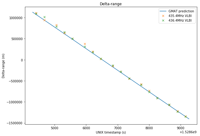
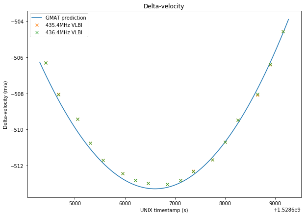
Note that the delta-range measurement is very noisy, since it uses “code measurements” and the code rate is only 250Hz. In fact, the estimates obtained in the two frequencies always differ by several tens of kilometers. In comparison, the delta-velocity measurement is very precise and both frequencies give almost the same result.
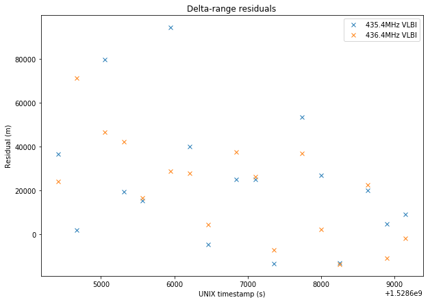
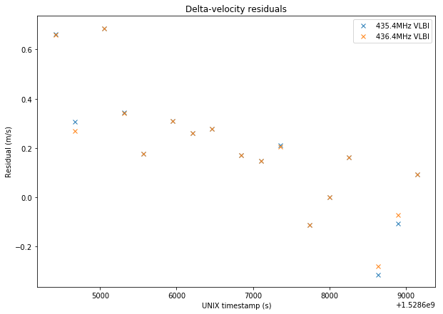
The plots below show the residuals, which are the difference between the measurements and the prediction by GMAT.
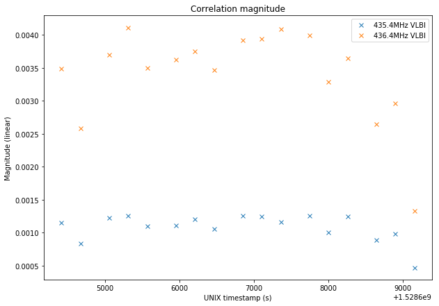
Finally, the plot below shows the magnitude of the correlation peak. We see that the strength of the signals remains more or less constant, but the 435.4Mhz signal is much weaker than the 436.4MHz signal. This effect has been already observed in most experiments and it is due to the attitude of DSWLP-B being unfavourable to the location of antenna A, according to the relative positions of the Earth, Moon and Sun (where DSWLP-B’s solar panel is pointing to during normal flight).
So far this is just a first look at the VLBI data. There is much experimentation that can be done and a lot of ideas that can be applied to this data.
6 comments