Amateur VLBI experiment with LilacSat-2

On 23 February, Wei Mingchuan BG2BHC published on Twitter the first Amateur VLBI experiment. This consisted of a GPS-synchronized recording of signals from LilacSat-2 using USRPs in groundstations at Harbin and Chongqing, which are about 2500km apart. Wei has made a Github repository containing the recording (in MATLAB file format) and some signal processing in MATLAB. I have done some signal processing of my own with the recording and published my results in a Jupyter notebook. Here I describe some general aspects about VLBI and its use in Amateur radio, and some specific details of the signal processing I have done.

VLBI stands for very-long-baseline interferometry and it is a new concept for most Amateurs, since this is the first time that VLBI is used in Amateur radio. Interferometry, in general, involves measuring some property about a radio (or optical) source using two or more receivers in different locations and then comparing the signals recorded at each receiver. The “baseline” refers to the distance (or the line segment) between the two receivers. Here, very-long refers to distances larger than a few kilometres, and usually hundreds or thousands of kilometres. This distinction is important for two reasons: first, using a long baseline gives more accuracy, as we will shortly see; second, interferometry requires synchronization between all receivers, and this has been historically quite difficult to achieve between distant receivers (today it is relatively easy using GPS).

For an example about how VLBI works, let us see the usual example in radio astronomy. Imagine a very distant radio source and two receivers on Earth. The radio wave from the source propagates in wave fronts which are almost planes, perpendicular to the direction of propagation. Therefore, the signal arrives to each receiver at different times. The
difference between the arrival times depends on the direction to the source with respect to the baseline (more precisely, on the angle between the direction to the source and the baseline), and also on the baseline length. In this way, the location of the source on the sky can be measured and tracked. Longer baselines give larger differences of arrival times, allowing a more precise measurement.

The case of LilacSat-2 is different to the situation described above, since it is a LEO satellite, not a very distant object. Therefore, instead of measuring its position in the sky, VLBI measures something called delta-range. This is just the difference of distances between the satellite and each of the groundstations. Another important measurement is delta-velocity. This is just the difference of velocities seen by each of the groundstations, or the time derivative of the delta-range. However, it is considered a different measurement because it is normally computed from phase measurements, rather than using times of arrival, as delta-range does. Using several delta-range or delta-velocity observations, either from different pairs of groundstations or from the same pair at different times, the position and velocity of the satellite can be estimated, and orbit determination can be done.

In fact, the main goal for the Harbin Amateur VLBI program is to perform orbit determination for the future DSLWP lunar mission (which I’ve talked about in a previous post). Since DSLWP will orbit outside the coverage of NORAD radars normally used for tracking near Earth objects, Amateur orbit determination via VLBI will be important for the mission.

The signal processing I have done with this experiment’s recording is described in my Amateur VLBI Jupyter notebook. Most of the techniques I’m using come from GNSS signal processing, since it is quite similar to this kind of VLBI.

The recording was made during a southbound pass of LilacSat-2 over China. It is quite short (around 30 seconds), since the common window when LilacSat-2 is visible from both groundstations is short, due to the long baseline in comparison with LilacSat-2’s orbit height.

A simple way to analyse the results of these measurements is to compare them with the values computed by using NORAD TLEs. The difference obtained is called residual, and it should be zero except for measurement errors (both in the VLBI measurements and in the TLEs, which are not very precise ephemeris), noise and so on. My results so far are quite good, as seen in the plots below.

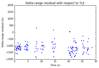
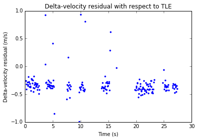
There is a bias in both delta-range and delta-velocity. This is probably partly because of some bias in the signal processing that can be corrected with some effort. Other than that, the measurement noise is really good. The delta-range noise is between 500 and 1000m, and the delta-velocity noise is around 0.25m/s.

The VLBI measurements are done using LilacSat-2’s 4k8 GFSK signal at 437.225MHz, which transmits telemetry packets. By doing a correlation of the signal received in each groundstation, the difference in times of arrival, and hence the delta-range can be calculated. A packet from this 4k8 GFSK signal is shown in the image below, taken from a post I wrote back in 2015.

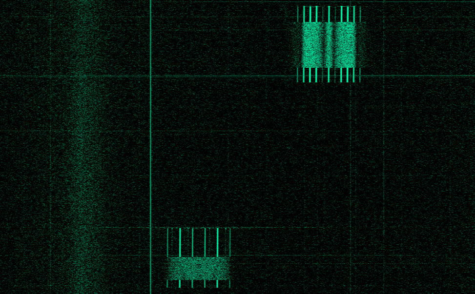
As you can see in the image, the 4k8 GFSK packets have a long preamble and postamble which consists of some periodic bits (which is what produces the spectral lines). This is not good for correlation, since a signal of short period will have closely spaced self-correlation peaks, producing an ambiguity in the delta-range measurement. A good signal for correlation is either aperiodic or has a long period. Usually, a PRN, such as a Gold code is used in GNSS because of this reason. The body of the 4k8 GFSK packet is scrambled with a CCSDS scrambler, so it provides a random-like signal that is good for performing correlation. Therefore, a valid measurement is only done while the body of a 4k8 GFSK packet is transmitted.

Although the signal processing techniques can be similar to those used in GNSS, some of the parameters are really different, giving new challenges for effective processing. The bits of the 4k8 signal are roughly 200 times longer than GPS chips (which have a frequency of 1.023MHz). In principle, this gives 200 times more noise in the delta-range measurement. The velocity of a LEO satellite is roughly 10 larger than that of a MEO GNSS satellite. This makes it more difficult using long integration times for the correlation (at least in open loop, as I’m doing here). The wavelength of the 70cm signal of LilacSat-2 is 3.6 times larger than that of an L-band GNSS satellite, giving 3.6 times more noise in the phase measurements (which is rather good in comparison with the large noise of delta-range measurements). However, since the frequency of the 4k8 GFSK signal is not precise, this gives an error when converting phase measurements to units of meters (this can contribute some bias to the delta-velocity shown above). It would be interesting to know how large is the error in frequency of the 4k8 GFSK signal.

I still have to study carefully the biases I’ve observed in my calculations, and I also have some ideas to improve my signal processing. However, I’ve decided to release the calculations I’ve done so far and write this post now, given the interest that this topic has sparked recently. Stay tuned for a future post with improved computations.