For a long time, AMSAT-DL has been using the 20 meter antenna in Bochum observatory to receive some telemetry from Tianwen-1, the Chinese Mars orbiter, almost daily. Since the telemetry includes the spacecraft’s state vectors, we can use this to monitor the spacecraft’s orbit. In 8 November 2021, Tianwen-1 entered its remote sensing orbit. This is an elliptical orbit with a period approximately 2/7 Mars sidereal days plus 170 seconds. This causes a ground track that is almost repeating, but drifts slowly to cover all the surface area of the planet.
I have been posting yearly updates about Tianwen-1’s orbit, the last of them this summer. In these updates, we can see that no manoeuvres have happened, and the changes in the Keplerian elements correspond to orbital perturbations caused by external forces. The orbit is in fact designed to cause the latitude of the periapsis to precess. In this way, all the surface of Mars can be scanned from low altitude.
Now we have some news. In the telemetry of the last few days we have detected that Tianwen-1 has raised its apoapsis radius from about 14134 km to 14489 km. All the data we have indicates that a propulsive burn has happened recently. In this post I give the details about this apoapsis raise manoeuvre.
This post is a continuation of my series about the 5G NR RAN. In these posts, I’m analyzing a recording of the downlink of an srsRAN gNB in a Jupyter notebook written from scratch. In this post I will show how to decode the PBCH (physical broadcast channel). The PBCH contains the MIB (master information block). It is transmitted in the SSB (synchronization signals / PBCH block). After detecting and measuring the synchronization signals, a UE must decode the PBCH to obtain the MIB, which contains some parameters which are essential to decode other physical downlink channels, including the PDSCH (physical downlink shared channel), which transmits the SIBs (system information blocks).
In my first post in the series, I already demodulated the PBCH. Therefore, in this post I will continue from there and show how to decode the MIB from the PBCH symbols. First I will give a summary of the encoding process. Decoding involves undoing each of these steps. Then I will show in detail how the decoding procedure works.
You might remember that back in July I made a recording of the DME ground-to-air and air-to-ground frequencies for a nearby VOR-DME station. In that post, I performed a preliminary analysis of the recording. I mentioned that I was interested in measuring the delay between the signals received directly from the aircraft and the ground transponder replies, and match these to the aircraft trajectories. This post is focused on that kind of study. I will present a GNU Radio out-of-tree module gr-dme that I have written to detect and measure DME pulses, and show a Jupyter notebook where I match aircraft pulses with their corresponding ground transponder replies and compare the delays to those calculated from the aircraft positions given in ADS-B data.
This year I submitted a track of challenges called “Not-LoRa” to the GRCon 2024 Capture The Flag. The idea driving this challenge was to take some analog voice signals and apply chirp spread spectrum modulation to them. Solving the challenge would require the participants to identify the chirp parameters and dechirp the signal. This idea also provided the possibility of hiding weak signals that are below the noise floor until they are dechirped, which is a good way to add harder flags. This blog post is an in-depth explanation of the challenge. I have put the materials for this challenge in this Github repository.
To give participants a context they might already be familiar with, I took the chirp spread spectrum parameters from several common LoRa modulations. These ended up being 125 kHz SF9, SF11 and SF7. LoRa is somewhat popular within the open source SDR community, and often there are LoRa challenges or talks in GRCon. This year was no exception, with a Meshtastic packet in the Signal Identification 7 challenge, and talks about gr-lora_sdr and Meshtastic_SDR.
DME (distance measuring equipment) is an aircraft radio navigation system that is used to measure the distance between an aircraft and a DME station on ground. DME is often colocated with a VOR station, in which case the VOR provides the bearing information. DME works by measuring the two-way time of flight of pulse pairs, which are first transmitted by the aircraft, then retransmitted with a fixed delay by the ground station, which acts as a transponder, and finally received back by the aircraft. DME operates between 960 and 1215 MHz. It is channelized in steps of 1 MHz, and the air-to-ground and ground-to-air frequencies always differ by 63 MHz (here is a list of all the frequency channels).
I want to write a post explaining in detail how DME works by analysing a recording of DME that contains both the air-to-ground and the ground-to-air channels. Among other things, I want to show that the delay between the aircraft and ground station pulses matches the one calculated using the aircraft position (which I can get from ADS-B data on the internet), the ground station position, the position of the recorder, and the fixed delay applied by the ground station transponder.
Recording two channels 63 MHz apart is tricky with the kind of SDRs I have. Devices based on the AD9361 technically support a maximum sample rate of 61.44 Msps (although some people are running it at up to 122.88 Msps). The LMS7002M, which is used by the LimeSDR and other SDRs, is an interesting alternative, for two reasons. First, it supports more than 61.44 Msps. However, it isn’t clear what is the maximum sample rate supported by the LimeSDR. Some sources, including the LimeSDR webpage mention 61.44 MHz bandwidth, but the LMS7002M datasheet says that the maximum RF modulation bandwidth (whatever that means) through the digital interface in SISO mode is 96 MHz. In the case of the LimeSDR there is also the limitation of the USB3 data rate, but this should not be a problem if we use only 1 RX channel. I haven’t found clear information about the limitations of each of the components of the LMS7002M (ADC max sample rate, etc.).
The second interesting feature is that the LMS7002M has a DDC on the chip. The AD9361 has a series of decimating filters to reduce the ADC sample rate and deliver a lower sample rate through the digital interface. The LMS7002M, in addition to this, has an NCO and digital mixer that can be be used to apply a frequency shift to the ADC IQ signal before decimation.
I had two different ideas about how to use the LimeSDR to record the two DME channels. The first idea consisted in using a 70 Msps output sample rate. For this I used an ADC sample rate of 140 Msps, because I think it is necessary to have at least decimation by 2 after the ADC (the LMS7200M documentation does not explain this clearly, so figuring out how to use the chip often involves some trial and error using LimeSuiteGUI). This idea had two problems. The first problem is that some CGEN PLL occasionally failed to lock when using an ADC sample rate of 140 Msps. However the LimeSuite driver retried multiple times until the PLL locked, so in practice this wasn’t a problem. This approach worked well on my desktop PC, since in 70 Msps I had the two DME channels and then I could use GNU Radio to extract each of the two channels (for instance with the Frequency Xlating FIR Filter). However, the laptop I planned to use to record on the field couldn’t keep up with 70 Msps.
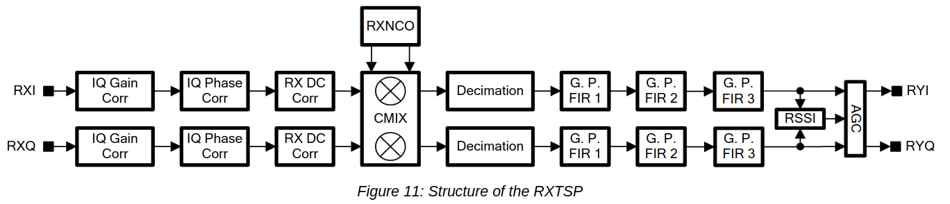
The second idea was to use the on-chip DDC in the LMS7200M to extract the DME channel and deliver a much lower sample rate over the digital interface. The figure below shows how the LMS7200M digital signal processing datapath works. This datapath is called RXTSP. The RXI and RXQ signals are the digital signals coming from the ADC (here and below, by ADC I mean a dual-channel ADC, since the LMS7002M is a zero-if IQ transceiver). The RYI and RYQ are the signals delivered to the digital interface of the chip. Since the LMS7200M has two RX channels, there are two identical chains, one for each channel. The parameters of each chain can be programmed completely independently.
LMS7200M digital signal processing, extracted from the datasheet
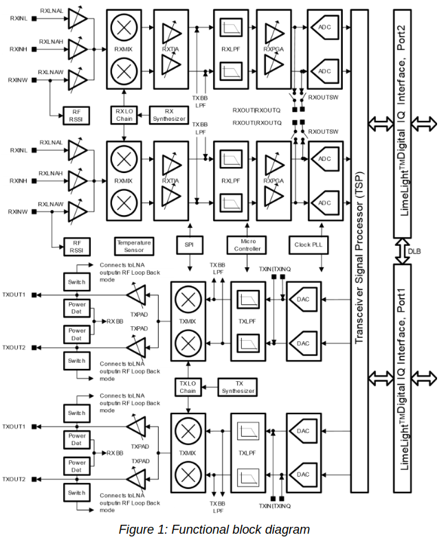
There is no way of sending the signal of one ADC to the two RXTSPs. The connection between each ADC and its corresponding RXTSP is fixed. Therefore, we need to feed in the antenna signal through the two RX channels, but we can easily do this with an external splitter. Remember that both of the LMS7200M RX channels share the same LO, as illustrated by the block diagram below. So the point here is to tune the LO to a frequency between the two DME channels, set the sample rate high enough that both DME channels are present in the ADC output, and finally to use each of the two RXTSPs to extract one of the DME channels, sending it at a low sample rate through the digital interface.
LMS7200M block diagram, extracted from the datasheet
This approach has worked quite well. I have set the ADC to 80 Msps and used the RXTSPs to dowconvert and decimate the DME channels to 2.5 Msps, recording that data directly in GNU Radio.
This post belongs to my series about LTE. In the LTE uplink, the PUSCH (physical uplink shared channel) is the channel used to trasmit data from the UEs (phones) to the eNB (base station). It plays a role analogous to the PDSCH (physical downlink shared channel), which is used to transmit data in the downlink. In this post I will decode the PUSCH in a recording that I made of my phone uplink a couple years ago.
The PUSCH uses the same kind of techniques as the PDSCH for transport block coding, so all the Turbo code implementation and related algorithms from my post about the PDSCH will be re-used here. However, there is an important difference between the PDSCH and the PUSCH that makes decoding the PUSCH much harder. The LTE downlink is, in a certain sense, a self-descriptive signal. The UEs don’t know in advance the configuration that will be used to transmit each transport block in the PDSCH, because the eNB decides it on the fly. Therefore, the eNB announces PDSCH transmissions in the PDCCH (physical downlink control channel).
When I decoded the PDCCH and PDSCH, the only slightly clever thing that I had to do was to find the RNTIs (radio network temporary indicators). These are 16-bit numbers that are used to address each PDSCH transmission. There are some of them which are statically allocated to some broadcast purpose (SI-RNTI, P-RNTI, RA-RNTI), and the C-RNTIs, which are individually assigned to each UE. The CRC-16 of the PDCCH DCIs is XORed with the RNTI to which the transmission is addressed. At any time, a UE knows the set of RNTIs that it is monitoring, so it calculates the CRC-16 of the received DCI, computes its XOR with each of its assigned RNTIs, and compares the result with the CRC-16 in the DCI. If there is a match, the DCI is accepted. This is a way of filtering out messages without spending additional bits to put the RNTI in a field in the DCI.
When we are monitoring an LTE downlink, we don’t know which RNTIs are being used. With some cleverness, if the SNR is good enough, we can detect and select each PDCCH transmission by hand (it is necessary to guess the REGs that it occupies and the DCI length) and then, assuming that we have decoded the DCI with no bit errors, obtain the RNTI as the XOR of the calculated CRC and the received CRC. This is what I did in the post about the PDCCH. If we were monitoring the LTE downlink for a longer time, this trick wouldn’t even be necessary. The C-RNTIs assigned to the UEs are communicated to them in a RAR transmitted with the RA-RNTI, as a response to their PRACH (see the post where I analyze this in Wireshark). So a downlink monitor application can simply watch the SI-RNTI, P-RNTI and RA-RNTI, and add any C-RNTIs to a list of known connected UEs when it sees a RAR. The C-RNTIs can be removed from this list after a period of inactivity, because the UE would have been sent to the idle state by the network. This idea really shows that it is possible to decode everything in the LTE downlink without doing clever blind decoding tricks.
In contrast, the LTE uplink is not self-descriptive. The eNB defines the configuration of each PUSCH transmission when it sends the uplink grant to the UE. So the UE doesn’t need to communicate this configuration again to the eNB when it transmits in the PUSCH. The information that describes the PUSCH transmissions is effectively in the PDCCH in the downlink, and in this case I don’t have a recording of the downlink that matches my uplink recording. This makes decoding the PUSCH much more difficult, but nevertheless not impossible. With some clever ideas and blind decoding tricks we can usually find all the information we’re missing. In the rest of this post, I describe how to do this in detail. It will be long and quite technical.
ERMINAZ-1U and ERMINAZ-1V are upcoming 1P PocketQubes by AMSAT-DL that will be launched in Rocket Factory Augsburg first flight from SaxaVord (Shetland, UK) later this year, together with other PocketQubes from AMSAT-EA and Libre Space Foundation. The ERMINAZ-1 satellites are based on the Libre Space QUBIK design and use the same communications system. Recently I have added a decoder for the ERMINAZ-1 satellites to gr-satellites and tested it using some pre-flight recordings that the team has shared with me.
The QUBIK communications stack uses something know as OSDLP (Open Space Data Link Protocol), which was developed by Libre Space based on CCSDS. Unfortunately, there is not much documentation about OSDLP. The best I’ve found are these slides, which only speak about the Data Link and higher layers. A look at the QUBIK transceiver GNU Radio flowgraph that AMSAT-DL is using with these satellites, together with some gr-satnogs blocks used in the flowgraph has been quite useful to figure out how the Synchronization and Coding layer of QUBIK works. In the rest of this post I will document my findings.
LTE-M is a family of several configurations supported by LTE for machine-to-machine and IoT communications. In this post I will talk specifically about BL/CE (bandwidth reduced low complexity / coverage enhancement), which is also known as LTE Cat M1. The main difference between a BL/CE UE and a regular LTE UE is that a BL/CE UE only supports a bandwidth of 1.4 MHz (in practice, 6 resource blocks, or 1.08 MHz) and can be half-duplex. These limitations reduce the cost, size and power of the UE, but require additional techniques to handle them.
If we think about the downlink, there are several signals that occupy the whole cell bandwidth, which is usually larger than 1.4 MHz. These are the PDCCH (physical downlink shared channel), the PCFICH (physical control format indicator channel) and the PHICH (physical hybrid-ARQ indicator channel). A BL/CE UE cannot receive any of these, so alternative signals must be used to provide similar functionality. Additionally, a BL/CE UE needs guard intervals in the time domain to support retuning of the 1.4 MHz slice in which the UE operates, and transmit/receive switching for half-duplex UEs. Another distinguishing feature of BL/CE is that messages are often repeated multiple times in order to support working with worse signal conditions than what is possible with a regular UE.
In LTE, the PSS and SSS (primary synchronization signal and secondary synchronization signal), as well as the PBCH (physical broadcast channel) occupy the central 6 resource blocks, so a BL/CE UE can synchronize to the cell and decode the MIB transmitted in the PBCH. The next step that a regular UE would perform is to monitor the PDCCH, first to find a SIB1 transmission (which is transmitted in the PDSCH), and then the rest of the SIBs (whose transmission schedule is listed in the SIB1). A BL/CE UE cannot do this, because it cannot receive the PDCCH and because the SIB PDSCH transmissions might be wider than 6 resource blocks. Therefore, in a cell that supports BL/CE UEs there are also SIB-BRs (BR stands for bandwidth reduced), which BL/CE UEs use instead of the regular SIBs. The SIB-BRs occupy 6 resource blocks and do not require receiving the PDCCH to be decoded. In this post I will use my recording of an LTE eNB to show how to decode the SIB-BRs, and other important aspects of BL/CE UEs.
I have implemented an FPGA DDC (digital downconverter) in Maia SDR. Intuitively speaking, a DDC is used to select a slice of the input spectrum. It works by using an NCO and mixer to move to the centre of the slice to baseband, and then applying low-pass filtering and decimation to reduce the sample rate as desired (according to the bandwidth of the slice that is selected).
At the moment, the output of the Maia SDR DDC can be used as input for the waterfall display (which uses a spectrometer that runs in the FPGA) and the IQ recorder. Using the DDC allows reaching sample rates below 2083.333 ksps, which is the minimum sample rate that can be used with the AD936x RFIC in the ADALM Pluto (at least according to the ad9361 Linux kernel module). Therefore, the DDC is useful to monitor or record narrowband signals. For instance, using a sample rate of 48 ksps, the 400 MiB RAM buffer used by the IQ recorder can be used to make a recording as long as 36 minutes in 16-bit integer mode, or 48 minutes in 12-bit integer mode. With such a sample rate, the 4096-point FFT used in the waterfall has a resolution of 11.7 Hz.
In the future, the DDC will be used by receivers implemented on the FPGA, both for analogue voice signals (SSB, AM, FM), and for digital signals. Additionally, I also have plans to allow streaming the DDC IQ output over the network, so that Maia SDR can be used with an SDR application running on a host computer. It is possible to fit several DDCs in the Pluto FPGA, so this would allow tuning independently several receivers within the same window of 61.44 MHz of spectrum. In the rest of this post I describe some technical details of the DDC.
In my previous posts I have been decoding LTE PDSCH (physical downlink shared channel) transmissions from an IQ recording of an eNB and looking at the MAC PDUs with Wireshark. The analysis I have done of the upper layer protocols is somewhat limited because I have decoded only 500 ms of traffic and because I don’t have the encryption keys, and also because I’m just beginning to learn how the LTE upper layers work. When doing this analysis I thought that it would be good to have a more complete example that I could use as a reference. A Google search for examples of PCAP files containing LTE MAC PDUs yields very little, so I thought I would make my own example with srsRAN. In this post I show how to set up an srsRAN LTE eNB and UE communicating over ZMQ on a single machine and then analyze the traffic in Wireshark.