Back in September, I showed how to decode the telemetry signal from Voyager 1 using a recording made with the Green Bank Telescope in 2015 by the Breakthrough Listen project. The recording was only 22.57 seconds long, so it didn’t even contain a complete telemetry frame. To study the contents of the telemetry, more data would be needed. Often we can learn things about the structure of the telemetry frames by comparing several consecutive frames. Fields whose contents don’t change, counters, and other features become apparent.
Some time after writing that post, Steve Croft, from BSRC, pointed me to another set of recordings of Voyager 1 from 16 July 2020 (MJD 59046.8). They were also made by Breakthrough Listen with the Green Bank Telescope, but they are longer. This post is an analysis of this set of recordings.
How to compute the symbol error rate rate of an m-FSK modulation is something that comes up in a variety of situations, since the math is the same in any setting in which the symbols are orthogonal (so it also applies to some spread spectrum modulations). I guess this must appear somewhere in the literature, but I can never find this result when I need it, so I have decided to write this post explaining the math.
Here I show an approach that I first learned from Wei Mingchuan BG2BHC two years ago during the Longjiang-2 lunar orbiter mission. While writing our paper about the mission, we wanted to compute a closed expression for the BER of the LRTC modulation used in the uplink (which is related to \(m\)-FSK). Using a clever idea, Wei was able to find a formula that involved an integral of CDFs and PDFs of chi-squared distributions. Even though this wasn’t really a closed formula, evaluating the integral numerically was much faster than doing simulations, specially for high \(E_b/N_0\).
Recently, I came again to the same idea independently. I was trying to compute the symbol error rate of \(m\)-FSK and even though I remembered that the problem about LRTC was related, I had forgotten about Wei’s formula and the trick used to obtain it. So I thought of something on my own. Later, digging through my emails I found the messages Wei and I exchanged about this and saw that he had arrived to the same idea and formula. Maybe the trick was in the back of my mind all the time.
Due to space constraints, the BER formula for LRTC and its mathematical derivation didn’t make it into the Longjiang-2 paper. Therefore, I include a small section below with the details.
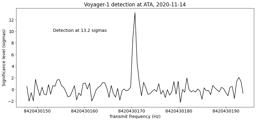
This post has been delayed by several months, as some other things (like Chang’e 5) kept getting in the way. As part of the GNU Radio activities in Allen Telescope Array, on 14 November 2020 we tried to detect the X-band signal of Voyager-1, which at that time was at a distance of 151.72 au (22697 millions of km) from Earth. After analysing the recorded IQ data to carefully correct for Doppler and stack up all the signal power, I published in Twitter the news that the signal could clearly be seen in some of the recordings.
Since then, I have been intending to write a post explaining in detail the signal processing and publishing the recorded data. I must add that detecting Voyager-1 with ATA was a significant feat. Since November, we have attempted to detect Voyager-1 again on another occasion, using the same signal processing pipeline, without any luck. Since in the optimal conditions the signal is already very weak, it has to be ensured that all the equipment is working properly. Problems are difficult to debug, because any issue will typically impede successful detection, without giving an indication of what went wrong.
I have published the IQ recordings of this observation in the following datasets in Zenodo:
In May 25, the Moon passed through the beam of my QO-100 groundstation and I took the opportunity to measure the Moon noise and receive the Moonbounce 10GHz beacon DL0SHF. A few days ago, in July 22, the Moon passed again through the beam of the dish. This is interesting because, in contrast to the opportunity in May, where the Moon only got within 0.5º of the dish pointing, in July 22 the Moon passed almost through the nominal dish pointing. Also, incidentally this occasion has almost coincided with the 50th anniversary of the arrival to the Moon of Apollo 11, and all the activities organized worldwide to celebrate this event.
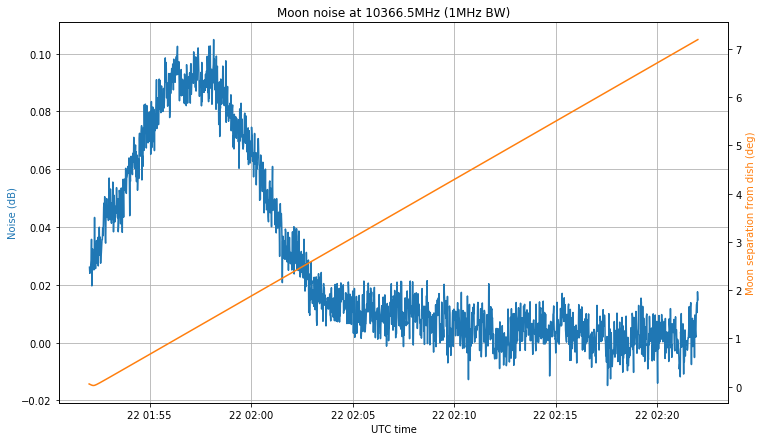
The figure below shows the noise measurement at 10366.5GHz with 1MHz and a 1.2m offset dish, compared with the angular separation between the Moon and the nominal pointing of the dish (defined as the direction from my station to Es’hail 2). The same recording settings as in the first observation were used here.
The first thing to note is that I made a mistake when programming the recording. I intended to make a 30 minute recording centred at the moment of closest approach, but instead I programmed the recording to start at the moment of closest approach. The LimeSDR used to make the recording was started to stream one hour before the recording, in order to achieve a stable temperature (this was one lesson I learned from my first observation).
The second comment is that the maximum noise doesn’t coincide with the moment when the Moon is closest to the nominal pointing. Luckily, this makes all the noise hump fit into the recording interval, but it means that my dish pointing is off. Indeed, the maximum happens when the Moon is 1.5º away from the nominal pointing, so my dish pointing error is at least 1.5º. I will try adjust the dish soon by peaking on the QO-100 beacon signal.
The noise hump is approximately 0.085dB, which is much better than the 0.05dB hump that I obtained in the first observation. It may not seem like much, but assuming the same noise in both observations, this is a difference of 2.32dB in the signal. This difference can be explained by the dish pointing error.
The recording I have made also covers the 10GHz Amateur EME band, but I have not been able to detect the signal of the DL0SHF beacon. Perhaps it was not transmitting when the recording was made. I have also arrived to the conclusion that the recording for my first observation had severe sample loss, as it was made on a mechanical hard drive. This explains the odd timing I detected in the DL0SHF signal.
The next observation is planned for October 11, but before this there is the Sun outage season between September 6 and 11, in which the Sun passes through the beam of the dish, so that Sun noise measurements can be performed.
Since I wasn’t going to be at home at that time, I programmed my computer to make a recording for later analysis. I recorded 4MHz of spectrum centred at 10367.5MHz using a LimeSDR connected to the LNB that I use to receive QO-100. The recording was planned to be 30 minutes long starting at 20:01 UTC, but for some reason only approximately 27 minutes were recorded.
This kind of events can be used to measure Moon noise and receive 10GHz EME signals. This post is an analysis of my recording, looking at these two things.
Yesterday, AMSAT-DLannounced that the narrowband transponder of QO-100 was under maintenance and that some changes to its settings would be made. This was also announced by the messages of the 400baud BPSK beacon. Not much information was given at first, but then they mentioned that the transponder gain was reduced by 6dB and a few hours later the beacon power was increased by 5dB.
Since I am currently doing continuous power measurements of the transponder noise and the beacons, when I arrived home I could examine the changes and determine using my measurements that the transponder gain was reduced by 5dB (not 6dB) at around 15:30 UTC, and then the uplink power of the beacons was increased by 5dB at around 21:00 UTC, thus bringing the beacons to the same downlink power as before. In what follows, I do a detailed analysis of my measurements.
I have replaced the dish I had for receiving Es’hail 2 by a new one. The former dish was a 95cm offset from diesl.es which was a few years old. I had previously used this dish for portable experiments, and it had been lying on an open balcony for many months until I finally installed it in my garden, so it wasn’t in very good shape.
Comparing with other stations in Spain, I received less transponder noise from the narrowband transponder of QO-100 than other stations. Doing some tests, I found out that the dish was off focus. I could get an improvement of 4dB or so by placing the LNB a bit farther from the dish. This was probably caused by a few hits that the dish got while using it portable. Rather than trying to fix this by modifying the arm (as the LNB couldn’t be held in this position), I decided to buy a new dish.
In the QO-100 (Es’hail 2) narrow band transponder, the recommendation for the adjustment of your downlink signal power is not to be stronger than the beacon. This was also the recommended usage of the old AO-40. Since the transponder has two beacons marking the transponder edges: a CW beacon marking the lower edge and a 400baud BPSK beacon marking the upper edge, there has been some debate on Twitter about which beacon does this recommendation refer to and what does “stronger” mean.
Of course, more formally, signal strength means power, which is a well defined physical concept, so there should be no argument about what does power mean. However, there are two different power measurements used for RF: average power and peak envelope power. I will assume that the recommendation refers to average power, not to peak envelope power. This makes more sense from the point of view of the power budget of the satellite amplifier (The total average power it needs to deliver is just the sum of the average powers of the signals of all the users, while the behaviour of the peak envelope power is much more complicated).
Also, I think that using peak envelope power for this restriction would be a very strict requirement on high PAPR signals. Note that the PAPR of CW is 0dB and the PAPR of BPSK is between 2 and 3dB, depending on the pulse shaping, so these are rather low PAPRs. For comparison, a moderately compressed SSB voice signal has a PAPR of 6dB.
In my opinion, the main problem with these discussions about “signal strength” is that many people are trying to judge power by looking at their waterfall or spectrum display and seeing what signal looks “higher”. This kind of measurement is not any good, because it doesn’t take signal bandwidth into account, depends on the FFT size, the window function, etc. It doesn’t help that many popular SDR software don’t have a good signal meter displaying the average power of the signal tuned in the passband.
In any case, I was curious about whether the power of the two beacons is the same and whether there is any interesting change over time. I have made a GNU Radio flowgraph that measures the power of each of the two beacons and of the transponder noise, and saves them to a file for later analysis.
David Rowe always insists that you should simulate the bit error rate for any modem you build. I’ve been intending to do some simulations of the decoders in gr-satellites since a while ago, and I’ve finally had some time to do so. I have simulated the performance of the LilacSat-1 decoder, both for uncoded BPSK and for the Viterbi decoder. This is just the beginning of the story, as the code can be adapted to simulate other modems. Here I describe some generalities about BER simulation in GNU Radio, the simulations I have done for LilacSat-1, and the results.
Leif’s generator is very simple. It uses a 555 timer to generate a square wave, a 74AC74 flip-flop to divide the frequency of the square wave by 2 and obtain a precise 50% duty cycle, a 74AC04 inverter as a driver, and capacitive coupling to turn the edges of the square wave into RF pulses. Alex’s SIGP-1 is an improvement over Leif’s design. It generates the square wave in the same manner, but then it uses a helical bandpass filter for 144MHz with around 5MHz bandwidth to convert the square wave into 144MHz pulses, and a PGA-103+ MMIC RF amplifier and a BFR91 RF NPN transistor as a class A amplifier to increase the output level. The SIGP-1 has two main advantages over Leif design. The output is stronger, so the S/N of the pulses is higher, and the filtering helps prevent saturation in the receiver. However, Leif’s design uses only simple components and it’s adequate in many cases.
I have built and tested Leif’s generator and used it to calibrate my FUNcube Dongle Pro+ at 144MHz. I’ve also tried doing the calibration at other frequencies and it also works well, but the pulses are not very strong at 432MHz and above.