dsp – Page 5 – Daniel Estévez

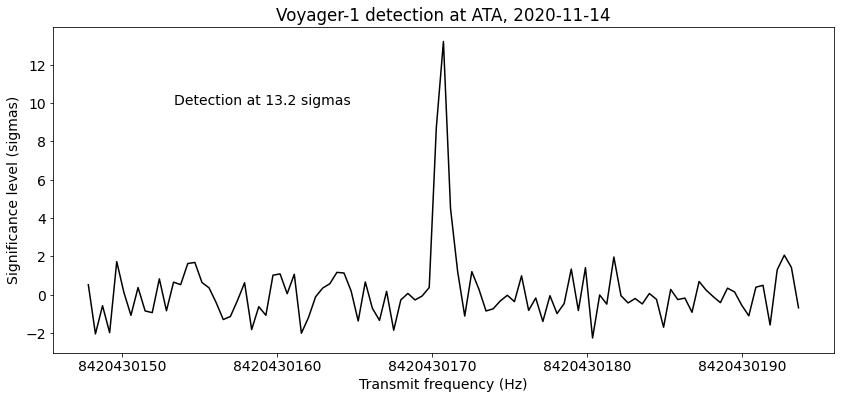
DSLWP-B first JT4G test

Yesterday, between 9:00 and 11:00, DSLWP-B made its first JT4G 70cm transmissions from lunar orbit. Several stations such as Cees Bassa and the rest of the PI9CAM team at Dwingeloo, the Netherlands, Fer IW1DTU in Italy, Tetsu JA0CAW and Yasuo JA5BLZ in Japan, Mike DK3WN in Germany, Jiang Lei BG6LQV in China, Dave G4RGK in the UK, and others exchanged reception reports on Twitter. Some of them have also shared their recordings of the signals.

Last week I presented a JT4G detection algorithm intended to detect very weak signals from DSLWP-B, down to -25dB SNR in 2500Hz. I have now processed the recordings of yesterday’s transmissions with this algorithm and here I look at the results. I have also made a Python script with the algorithm so that people can process their recordings easily. Instructions are included in this post.

First results of DSLWP-B Amateur VLBI

In March this year I spoke about the Amateur VLBI with LilacSat-2 experiment. This experiment consisted of a GPS-synchronized recording of LilacSat-2 at groundstations in Harbin and Chongqing, China, which are 2500km apart. The experiment was a preparation for the Amateur VLBI project with the DSLWP lunar orbiting satellites, and I contributed with some signal processing techniques for VLBI.

As you may know, the DSLWP-B satellite is now orbiting the Moon since May 25 and the first Amateur VLBI session was performed last Sunday. The groundstations at Shahe in Beijing, China, and Dwingeloo in the Netherlands performed a GPS-synchronized recording of the 70cm signals from DSLWP-B from 04:20 to 5:40 UTC on 2018-06-10. I have adapted my VLBI correlation algorithms and processed these recordings. Here are my first results.

JT4G detection algorithm for DSLWP-B

Now that DSLWP-B has already been for 17 days in lunar orbit, there have been several tests of the 70cm Amateur Radio payload, using 250bps GMSK with an r=1/2 turbo code. Several stations have received and decoded these transmissions successfully, ranging from the 25m radiotelescope at PI9CAM in Dwingeloo, the Netherlands (see recordings here) and the old 12m Inmarsat C-band dish in Shahe, Beijing, to much more modest stations such as DK3WN‘s, with a 15.4dBic 20-element crossed yagi in RHCP. The notices for future tests are published in Wei Mingchuan BG2BHC’s twitter account.

As far as I know, there have been no tests using JT4G yet. According to the documentation of WSJT-X 1.9.0, JT4G can be decoded down to -17dB SNR measured in 2.5kHz bandwidth. However, if we don’t insist on decoding the data, but only detecting the signal, much weaker signals can be detected. The algorithm presented here achieves reliable detections down to about -25dB SNR, or 9dB C/N0.

This possibility is very interesting, because it enables very modest stations to detect signals from DSLWP-B. In comparison, the r=1/2 turbo code can achieve decodes down to 1dB Eb/N0, or 25dB C/N0. In theory, this makes detection of JT4G signals 16dB easier than decoding the GMSK telemetry. Thus, very small stations should be able to detect JT4G signals from DSLWP-B.

Improved signal processing for LilacSat-2 VLBI

Last week I published my results about the LilacSat-2 VLBI experiment. There, I mentioned that there were some things I still wanted to do, such as studying the biases in the calculations or trying to improve the signal processing. Since then, I have continued working on this and I have tried out some ideas I had. These have given good results. For instance, I have been able to reduce the delta-range measurement noise from around 700m to 300m. Here I present the improvements I have made. Reading the previous post before this one is highly recommended. The calculations of this post were performed in this Jupyter notebook.

Amateur VLBI experiment with LilacSat-2

On 23 February, Wei Mingchuan BG2BHC published on Twitter the first Amateur VLBI experiment. This consisted of a GPS-synchronized recording of signals from LilacSat-2 using USRPs in groundstations at Harbin and Chongqing, which are about 2500km apart. Wei has made a Github repository containing the recording (in MATLAB file format) and some signal processing in MATLAB. I have done some signal processing of my own with the recording and published my results in a Jupyter notebook. Here I describe some general aspects about VLBI and its use in Amateur radio, and some specific details of the signal processing I have done.

Mystery 9k6 BPSK satellite

On January 28th, Tetsu JA0CAW reported on Twitter his reception of an unknown satellite. The time of reception was 2018-01-28 12:15 UTC and the frequency was around 435.525MHz. The time and frequency coincided with a PicSat pass over JA0CAW’s station in Japan. He provided an IQ recording of the signal. So far, the satellite that originated the signal has not been identified. Several people have tried to listen to this satellite again, but I haven’t seen any other reports. Doppler identification has not been attempted and it is perhaps unfeasible with the few packets in JA0CAW’s recording.

I have looked at the recording to try to identify the satellite. The modulation is easily seen to be BPSK at 9600baud. The signal presents a lot of fading, so demodulation without bit errors is difficult. There seems to be a scrambler in use. I’ve tried descrambling with G3RUH and CCSDS without any luck. I’ve also failed to identify a preamble or frame sync marker.

To look at the packets in more detail, I’ve resorted to do demodulation as postprocessing in a Jupyter Python notebook. The resulting notebook is here. It is written with detailed comments, so it can be of interest to anyone who wants to learn these techniques.

The only interesting piece of information that I’ve been able to extract from my analysis is that the bits in the packets present strong self-correlations at lags of 1920 bits (and multiples). This is 240 bytes, but I have no clue of what to make of this.

As always, I would be grateful if anyone can provide any additional information about this unknown satellite.

Using CODAR for ionospheric sounding

CODAR is an HF radar used to measure surface ocean currents in coastal areas. Usually, it consists of a chirp which repeats every second. The chirp rate is usually on the order of 10kHz/s, and the signal is gated in small pulses so that the CODAR receiver can listen between pulses. The gating frequency can be on the order of 1kHz.

CODAR can be received by skywave many kilometers inland. Being a chirped signal, it is easy to extract the multipath information from the received signal. In this way, one can see the signal bouncing off the different layers of the ionosphere, and magnificent pictures showing the changes in the ionosphere (especially at dawn and dusk) can be obtained. For instance, see these images by Pieter Ibelings N4IP, or the image at the top of this post, which contains 48 hours worth of CODAR data.

Here I describe my approach to receiving CODAR. It uses GNU Radio for most of the signal processing, and Python with NumPy, SciPy and Matplotlib for plotting.

Polarization in Voyager signal from Green Bank Telescope

A few days ago I read the paper about the Breakthrough Listen experiment. This experiment consists in doing many wideband recordings of different stars using the Green Bank Telescope, and (in the future) Parkes Observatory and then trying to find signals from extraterrestrial intelligent life in the recordings. The Breakthrough Listen project has a nice Github repository with some documentation and an analysis of a recording they did of Voyager 1 to test their setup.

I have also been thinking about how to study the polarization of signals in a dual polarization recording (two coherent channels with orthogonal polarizations). My main goal for this is to study the polarization of the signals of Amateur satellites in low Earth orbit. It seems that there are many myths regarding polarization and the rotation of cubesats, and these myths eventually pop up whenever anyone tries to discuss whether linearly polarized or circularly polarized Yagis are any good for receiving cubesats.

Through the Breakthrough Listen paper I’ve learned of the Stokes parameters. These are a set of parameters to describe polarization which are very popular in optics, since they are easy to measure physically. I have immediately noticed that they are also easy to compute from a dual polarization recording. In comparison with Jones vectors, Stokes parameters disregard all the information about phase, but instead they are computed from the averaged power in different polarizations. This makes their computation less affected by noise and other factors.

As I also wanted to get my hands on the Breakthrough Listen raw recordings, I have been computing the Stokes parameters of the Voyager 1 signal in their recording. Since the Voyager 1 signal is left hand circularly polarized, the results are not particularly interesting. It would be better to use a signal with changing polarization or some form of elliptical polarization.

I have started to use Jupyter notebook. This is something I had been wanting to try since a while ago, and I’ve realised that a Jupyter notebook serves better to document my experiments in Python than a Python script in a gist, which is what I was doing before. I have started a Github repo for my experiments using Jupyter notebooks. The experiment about polarization in the Voyager 1 signal is the first of them. Incidentally, this experiment has been done near Voyager 1’s 40th anniversary.

AGC for gr-satellites

In a previous post I discussed my BER simulations with the LilacSat-1 receiver in gr-satellites. I found out that the “Feed Forward AGC” block was not performing well and causing a considerable loss in performance. David Rowe remarked that an AGC should not be necessary in a PSK modem, since PSK is not sensitive to amplitude. While this is true, several of the GNU Radio blocks that I’m using in my BPSK receiver are indeed sensitive to amplitude, so an AGC must be used with them. Here I look at these blocks and I explain the new AGC that I’m now using in gr-satellites.

Acquisition and wipeoff for JT9A

Lately, I have been playing around with the concept of doing acquisition and wipeoff of JT9A signals, using a locally generated replica when the transmitted message is known. These are concepts and terminologies that come from GNSS signal processing, but they can applied to many other cases.

In GNSS, most of the systems transmit a known spreading sequence using BPSK. When the signal arrives to the receiver, the frequency offset (given by Doppler and clock error) and delay are unknown. The receiver runs a search correlating against a locally generated replica signal which uses the same spreading sequence. The correlation will peak for the correct values of frequency offset and delay. The receiver then mixes the incoming signal with the replica to remove the DSSS modulation, so that only the data bits that carry the navigation message remain. This process can be understood as a matched filter that removes a lot of noise bandwidth. The procedure is called code wipeoff.

The same ideas can be applied to almost any kind of signal. A JT9A signal is a 9-FSK signal, so when trying to do an FFT to visually detect the signal in a spectrum display, the energy of the signal spreads over several bins and we lose SNR. We can generate a replica JT9A signal carrying the same message and at the same temporal delay than the signal we want to detect. Then we mix the signal with the complex conjugate of the replica. The result is a CW tone at the difference of frequencies of both signals, which we call wiped signal. This is much easier to detect in an FFT, because all the energy is concentrated in a single bin. Here I look at the procedure in detail and show an application with real world signals. Recordings and a Python script are included.