dsp – Page 6 – Daniel Estévez

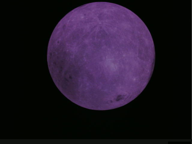
WSJT-X and linear satellites: part I

Several weeks ago, in an AMSAT EA informal meeting, Eduardo EA3GHS wondered about the possibility of using WSJT-X modes through linear transponder satellites in low Earth orbit. Of course, computer Doppler correction is a must, but even under the best circumstances we cannot assume a perfect Doppler correction. First, there are errors in the Doppler computation because the TLEs used are always measured at an earlier time and do not reflect exactly the current state of the satellite. This was the aspect that Eduardo was studying. Second, there are also errors because the computer clock is not perfect. Even a 10ms error in the computer clock can produce a noticeable error in the Doppler computation. Also, usually there is a delay between the time that the RF signal reaches the antenna and the time that the Doppler correction is computed for and applied to the signal, especially if using SDR hardware, which can have large buffers for the signal. This delay can be measured and compensated in the Doppler calculation, but this is usually not done.

Here we look at errors of the second kind. We denote by \(D(t)\) the function describing the Doppler frequency, where \(t\) is the time when the signal arrives at the antenna. We assume that the correction is not done using \(D(t)\), but rather \(D(t – \delta)\), where \(\delta\) is a small constant. Thus, a residual Doppler \(D(t)-D(t-\delta)\) is still present in the received signal. We will study this residual Doppler and how tolerant to it are several WSJT-X modes, depending on the value of \(\delta\).

The dependence of Doppler on the age of the TLEs will be studied in a later post, but it is worthy to note that the largest error made by using old TLEs is in the along-track position of the satellite, and that this effect is well modelled by offsetting the Doppler curve in time. This justifies the study of the residual Doppler \(D(t)-D(t-\delta)\).

Waterfalls from the EAPSK63 contest

Last weekend, I recorded the full EAPSK63 contest in the 40m band with the goal of monitoring IMD levels. I made a 48kHz IQ recording spanning the full 24 contest hours (from 16:00 UTC on Saturday to 16:00 UTC on Sunday). This week I’ve been playing with making waterfall plots from the recording. These are very interesting, showing patterns in propagation and contest activity. Here I show some of the waterfalls I’ve obtained, together with the Python code used to compute them.

Monitoring IMD levels in the EAPSK63 contest

This weekend I have recorded the full EAPSK63 Spanish PSK63 contest in the 40m band with the goal of playing back the recording later and reporting the stations showing excessively high IMD levels. In PSK contests, it is usual to see terribly distorted signals, which are the result of reckless operating techniques and stations which are setup inadequately. Contest rules don’t help much, as they are usually too weak to prevent distorted signals from interfering other participants. Amateurs should take care and strive to produce a signal as clean as possible. For instance, in the US, Part 97 101 a) states that “each amateur station must be operated in accordance with good engineering and good amateur practice”. Here I describe the signal processing done in this study and list a “hall of shame” of the worst stations I have spotted in my recording. I will notify by email the contest manager and all the stations in this list with the hope that the situation improves in the future.

Improving signal processing in my OTH radar receiver

This is a follow up post to my experiments studying OTH radar. I have found that the signal processing I did there to obtain the cross-correlation was far from optimal. This produced the strange side-bands below the main reflection. The keen reader might have noticed that I was doing the cross-correlation with a template pulse that lasted the whole pulse repetition cycle. However, the pulses from the radar are shorter. Therefore, it is a better idea to use a shorter template pulse. Ideally, the template pulse should have the same length as the transmitted pulse. However, I don’t know this length precisely, because multipath propagation makes the received pulses a bit longer. However, I think that 6.5ms is a good estimate.

I have also changed the window for the pulse. I’m now using a Dolph-Chebyshev window. I use scipy to compute this window, because it is not included in GNU Radio. This window has the property that the side-bands have constant attenuation. Indeed, it minimizes the \(L^\infty\) norm of the side-bands. There is a parameter that tunes the side-bands attenuation. For higher attenuations, you have a wider main lobe, while if you want a narrower main love you get less side-band attenuation. These properties make this window useful in radar applications.

Below I’m doing the cross-correlation in GNU Radio with a shorter template pulse shaped with a Dolph-Chebyshev window set for 55dB attenuation.

The good thing about the settable attenuation of the Dolph-Chebyshev window is that it can be used to trade-off performance between different features. First, we use an attenuation of 100dB. The side-bands are below the noise floor in this case, so we have no “false responses” in our cross-correlation. The drawback is that the main lobe is wide so the resolution of the features of the ionosphere in the image below is not very good.

Dolph-Chebyshev window with 100dB attenuation

Next we try with 55dB attenuation. This narrows the main lobe, improving the resolution and crispness of the features of the ionosphere in the image below. However, side-bands start being visible above the noise floor, producing “false responses”. However, comparing with the image above, we now know where the false responses are.

Dolph-Chebyshev window with 55dB attenuation

I have updated the gist with the GNU Radio flowgraph and python script used to produce the images.

Scramblers and their implementation in GNUradio

A scrambler is a function that is applied to a sequence of data before transmitting with the goal of making this data more “random-like”. For instance, scrambling avoids long runs of the bits 0 or 1 only, which may make the receiver loose synchronization or cause spectral concentration of the signal. The receiver applies the inverse function, which is called descrambler, to recover the original data. The documentation for the scrambler blocks in GNUradio is not very good and one may need to take a look at the implementation of these blocks to get their parameters right. Here, I’ll try to explain a bit of the mathematics behind scramblers and the peculiarities of their implementation in GNUradio.

Another look at recursive quadrature oscillators

In a recent post, we looked at which \(2\times 2\) Toeplitz real matrices \(T\) gave useful quadrature oscillators by the recurrence \(x_{n+1}=T x_n\). There, we computed their eigenvalues and solved the recurrence in terms of them. Of course, there are many other ways to approach this problem. Here we look at another approach that gives a good geometric picture of what happens, can be applied to general \(2\times 2\) matrices, and may be used as a starting point for the \(n\times n\) case.

A look at a new digital quadrature oscillator

Two sinusoidal signals are said to be in quadrature if they have a constant phase difference of 90º. Quadrature signals are widely used in signal processing. A digital quadrature oscillator is just an algorithm that computes the sequence \(x_n = (\cos(\omega n), \sin(\omega n))\), \(n\geq 0\), or a similar sequence of sinusoids in quadrature. Here \(\omega\) is the oscillator frequency in radians per sample. Direct computation of this sequence is very time consuming, because the trigonometric functions have to be evaluated for each sample. Therefore, it is a good idea to use a linear recurrence scheme to compute \(x_n\). Using basic trigonometric identities, we see that\[x_{n+1} = A x_n,\quad x_0=\begin{pmatrix}1\\0\end{pmatrix},\]with\[A = \begin{pmatrix}\alpha_1 & -\alpha_2\\\alpha_2 & \alpha_1\end{pmatrix},\quad \alpha_1 = \cos(\omega),\ \alpha_2=\sin(\omega).\]

However, to actually perform these computations in a digital processor, one has to quantize \(\alpha_1,\alpha_2\), meaning that one has to replace \(\alpha_1,\alpha_2\) by approximations. It is easy to see that if one replaces \(\alpha_1,\alpha_2\) by some perturbation, then the eigenvalues of \(A\) are no longer in the unit circle, so the oscillation can grow or decay exponentially and one would need to apply an AGC scheme to keep this method stable.

Here we will look at a new quadrature oscillator by Martin Vicanek that has appeared recently and solves this problem.