Last week I published my results about the LilacSat-2 VLBI experiment. There, I mentioned that there were some things I still wanted to do, such as studying the biases in the calculations or trying to improve the signal processing. Since then, I have continued working on this and I have tried out some ideas I had. These have given good results. For instance, I have been able to reduce the delta-range measurement noise from around 700m to 300m. Here I present the improvements I have made. Reading the previous post before this one is highly recommended. The calculations of this post were performed in this Jupyter notebook.
The most challenging part for processing this VLBI experiment is that the delta-velocity is quite high (around 11km/s). In comparison, in GNSS with MEO satellites, the maximum velocity projected onto the line of sight is around 800m/s. This very high delta-velocity causes several problems. The most important is that the delta-range changes roughly 740m during each of the FFT integrations I was doing (with \(N = 2^{14}\) samples). There are two main consequences of this. First, the measurements need to be time-tagged properly. Even mistaking the time tag by as little as \(N\) samples causes a large bias. Second, during the correlation via FFT, the correlation peak is moving. This causes the correlation peak to become smeared, making it more difficult to locate the correlation peak accurately. To put things in perspective, 740m is roughly 0.6 samples.
The solution to the first problem is to be careful and time-tag adequately all measurements. In my previous study I had been too careless about it, introducing biases due to improper tagging. Proper time-tagging is done as follows. Note that when we do an FFT correlation, the result of this correlation has to be tagged with the sample in the middle of the FFT interval. In fact, as we have already seen, the correlation peak moves 0.6 samples during the FFT interval. Therefore, the FFT correlation computes the average position of the correlation peak. This corresponds to the position of the peak at the middle of the FFT interval, since the velocity at which the peak travels is almost constant. Since we are doing FFT correlations for the samples \([0,N-1],[N,2N-1],\ldots\), we should time-tag these with the samples \(N/2, 3N/2,\ldots\).
This time tagging is adequate for the delta-range and phase measurements. However, delta-frequency and delta-velocity are computed by subtracting consecutive phase measurements (discrete differentiation). In other words, the difference between the phase at sample \(3N/2\) and the phase at sample \(N/2\) approximates the frequency at sample \(N\) (which is the midpoint of \(N/2\) and \(3N/2\)). Therefore, the delta-frequency and delta-velocity measurements should be time-tagged with the samples \(N,2N,\ldots\).
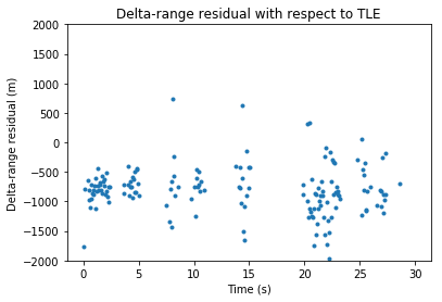
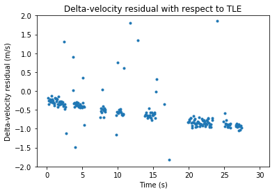
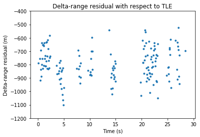
When doing the time-tags in this manner, we obtain the following residuals against the TLEs.
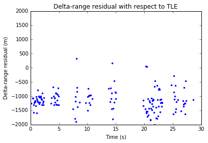
Compare with the residuals shown in the previous post, where everything was time-tagged with the samples \(0,N,\ldots\).
We see that the delta-range residual has decreased by roughly 500m. However, the delta-velocity now shows a small linear drift. It is difficult to judge whether this is a problem with the inaccuracy of the TLEs or some additional bias that the signal processing is introducing.
One solution to the second problem (the fact that the correlation peak moves during the correlation interval) is to resample one of the two signals according to the delta-velocity to try to keep the correlation peak in the same place during each correlation interval. In this way, the correlation peak doesn’t get smeared and the peak can be located more accurately. The drawback of this approach is that most useful applications of this idea require arbitrary resampling (or interpolation) of one of the signals.
In the algorithm I have designed, I am using sinc interpolation with the second signal (the one corresponding to the Harbin groundstation). I use the phase measurement obtained before to calculate how the Harbin signal should be resampled to keep the correlation peak in place during each correlation interval. This allows longer correlation intervals and makes peak location more accurate. The details of the algorithm are shown in the Jupyter notebook.
Another thing I’ve noted is that the peak estimation algorithm I used was not adequate. This peak estimation algorithm was used to get subsample resolution in the location of the correlation peak. The idea is that the sample with the largest correlation and its two adjacent samples are sent to the peak estimation algorithm. This then locates the peak by assuming that the shape of the peak is an isosceles triangle. It fits the triangle to the three data points and gets the position of the vertex (fitting is only done implicitly).
This idea is good for GNSS signals, which use rectangular shaping, so the correlation peak is in fact shaped as an isosceles triangle. However, for smooth pulse shaping, such as the Gaussian pulse shaping used in LilacSat-2, the correlation peak is a parabola. Therefore, I have designed a new peak estimation algorithm that fits a parabola through the three data points and gets the position of the vertex. The result obtained with this algorithm is only slightly different to the one that the triangle method gives, but keep in mind that slightly different here can mean a difference of 100 or 200m, since the distance between samples is roughly 1200m.
I have also played with the idea of sending more than three points into the peak estimator, and performing a least-squares fit for a parabola using all the points. However, the results are very similar to those obtained using only three points.
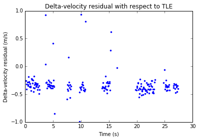
With the resampling algorithm and the parabola peak estimator, the following improved results for the delta-range can be obtained. Here I am using a coherent integration interval of roughly 1 second. The length of the interval doesn’t seem to be very critical, since the SNR is already quite good.
Note that the measurement noise is now around 300m. This is a noticeable improvement.