PW-Sat2 transmits standard G3RUH-scrambled BPSK AX.25 frames in the 70cm Amateur Satellite band. The baudrate can be selected between 1k2, 2k4, 4k8 and 9k6 by the satellite team. The interesting thing is that there are many types of packets besides telemetry. For instance, it can list and transfer on-board files, such as the images taken by the satellite camera. These packets can be decoded by using the FramePayloadDecoder software.
Since the FramePayloadDecoder software is quite complex and it is written in Python, I have decided to make a telemetry parser for gr-satellites that simply loads this software into GNU Radio and passes the frames to the decoder. Here are the instructions to set this up.
The communications system of 3CAT-1 uses a Texas Instrument CC1101 FSK transceiver chip, which is very similar to the CC1125 used in Reaktor Hello World. It transmits a 9k6 FSK telemetry beacon in the 70cm Amateur band. An interesting thing about this beacon is that it is powered by a temperature gradient that generates naturally within the satellite. A Peltier module is used to collect energy from the gradient and power the communications module. This is called “eternal self-powered beacon demonstrator” by the designers of the satellite, since it doesn’t depend on batteries or solar cells.
I have been in contact with Juan Fran Muñoz from NanoSat Lab, who has been kind enough to send me a telemetry recording for 3CAT-1. With this, and following my implementation of the Reaktor Hello World decoder, I have added a decoder for 3CAT-1 to gr-satellites.
Reaktor Hello World is a 2U cubesat built by the Finnish company Reaktor Space Lab as a test of their cubesat platform and demonstration of the first miniature infrared hyperspectral imager. It was launched on November 29 by a PSLV from Satish Dhawan Space Centre, together with several other cubesats. It transmits 9k6 GFSK telemetry in the 70cm Amateur satellite band.
The satellite uses a Texas Instruments CC1125 FSK transceiver chip. This is very similar to the CC1101 that I used a few years ago in my 70cm Hamnet experiments, so I already knew the coding and features of this chip quite well. The satellite team has a Github repository with a GNU Radio decoder based on the gr-cc11xx decoder block for the CC11xx series of chips. Since gr-cc11xx doesn’t seem to be maintained anymore, I wanted to implement my own CC11xx decoder in gr-satellites and use it to decode Reaktor Hello World.
However, so far the reflection has been detected by hand by looking at the recording waterfalls. We don’t have any statistics about how often it happens or which conditions favour it. I want to make some scripts to process all the Dwingeloo recordings in batch and try to extract some useful conclusions from the data.
Here I show my first script, which computes the power of the direct and reflected signals (if any). The analysis of the results will be done in a future post.
Lately, I have been testing the GPSDO that I will use to discipline my Es’hail 2 groundstation. One of the tests I have done is to measure the frequency of the TCXO that I use in my Hermes-Lite 2.0beta2 over a few days. Here I show the details of the measurement process and how to process the data in Python.
I have made a Python script to plot the Doppler and geometry for a DSLWP-B observation. This can be useful for several things: predicting the downlink and uplink Doppler corrections, checking for the Doppler of the Moonbounce signal, checking the position of DSLWP-B in the sky, and studying Moonbounce geometry.
While writing my previous report, I had to keep track of when each of the images had been taken and when it was downloaded. This can be a bit tricky, since the images do not carry a timestamp. Here I describe the techniques that can bee used to identify and keep track of the images.
The SiriusSats are using 4k8 FSK AX.25 packet radio at 435.570MHz and 435.670MHz respectively, using callsigns RS13S and RS14S. The Tanushas transmit at 437.050MHz. Tanusha-3 normally transmits 1k2 AFSK AX.25 packet radio using the callsign RS8S, but Mike Rupprecht sent me the other day a recording of a transmission from Tanusha-3 that he could not decode.
It turns out that the packet in this recording uses a very peculiar modulation. The modulation is FM, but the data is carried in audio frequency phase modulation with a deviation of approximately 1 radian. The baudrate is 1200baud and the frequency for the phase modulation carrier is 2400Hz. The coding is AX.25 packet radio.
Why this peculiar mode is used in addition to the standard 1k2 packet radio is a mystery. Mike believes that the satellite is somehow faulty, since the pre-recorded audio messages that it transmits are also garbled (see this recording). If this is the case, it would be very interesting to know which particular failure can turn an AFSK transmitter into a phase modulation transmitter.
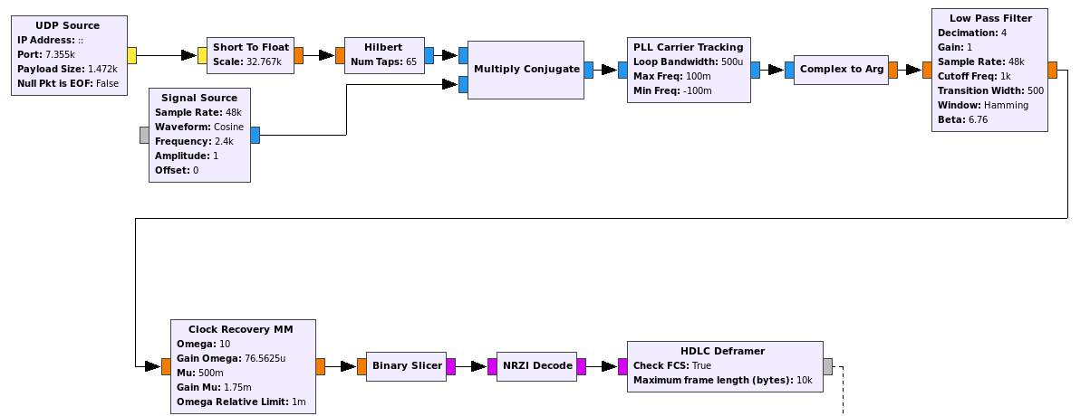
I have added support to gr-satellites for decoding the Tanusha-3 phase modulation telemetry. To decode the standard 1k2 AFSK telemetry direwolf can be used. The decoder flowgraph can be seen in the figure below.
TANUSHA-3 gr-satellites decoder
The FM demodulated signal comes in from the UDP source. It is first converted down to baseband and then a PLL is used to recover the carrier. The Complex to Arg block recovers the phase, yielding an NRZ signal. This signal is lowpass filtered, and then clock recovery, bit slicing and AX.25 deframing is done. Note that it is also possible to decode this kind of signal differentially, without doing carrier recovery, since the NRZI encoding used by AX.25 is differential. However, the carrier recovery works really well, because there is a lot of residual carrier and this is an audio frequency carrier, so it should be very stable in frequency.
The recording that Mike sent me is in tanusha3_pm.wav. It contains a single AX.25 packet that when analyzed in direwolf yields the following.
RS8S>ALL:This is SWSU satellite TANUSHA-3 from Russia, Kursk<0x0d>
------
U frame UI: p/f=0, No layer 3 protocol implemented., length = 68
 dest    ALL     0 c/r=1 res=3 last=0
 source  RS8S    0 c/r=0 res=3 last=1
  000:  82 98 98 40 40 40 e0 a4 a6 70 a6 40 40 61 03 f0  ...@@@...p.@@a..
  010:  54 68 69 73 20 69 73 20 53 57 53 55 20 73 61 74  This is SWSU sat
  020:  65 6c 6c 69 74 65 20 54 41 4e 55 53 48 41 2d 33  ellite TANUSHA-3
  030:  20 66 72 6f 6d 20 52 75 73 73 69 61 2c 20 4b 75   from Russia, Ku
  040:  72 73 6b 0d                                      rsk.
------
The contents of the packet are a message in ASCII. The message is of the same kind as those transmitted in AFSK.
If you’ve being following my latestposts, probably you’ve seen that I’m taking great care to decode as much as possible from the SSDV transmissions by DSLWP-B using the recordings made at the Dwingeloo radiotelescope. Since Dwingeloo sees a very high SNR, the reception should be error free, even without any bit error before Turbo decoding.
However, there are some occasional glitches that corrupt a packet, thus losing an SSDV frame. Some of these glitches have been attributed to a frequency jump in the DSLWP-B transmitter. This jump has to do with the onboard TCXO, which compensates frequency digitally, in discrete steps. When the frequency jump happens, the decoder’s PLL loses lock and this corrupts the packet that is being received (note that a carrier phase slip will render the packet undecodable unless it happens very near the end of the packet).
There are other glitches where the gr-dslwp decoder is at fault. The ones that I’ve identify deal in one way or another with the detection of the ASM (attached sync marker). Here I describe some of these problems and my proposed solutions.
Today an SSDV transmission session from DSLWP-B was programmed between 7:00 and 9:00 UTC. The main receiving groundstation was the Dwingeloo radiotelescope. Cees Bassa retransmitted the reception progress live on Twitter. Since the start of the recording, it seemed that some of the SSDV packets were being lost. As Dwingeloo gets a very high SNR and essentially no bit errors, any lost packets indicate a problem either with the transmitter at DSLWP-B or with the receiving software at Dwingeloo.
My analysis of last week’s SSDV transmissions spotted some problems in the transmitter. Namely, some packets were being cut short. Therefore, I have been closely watching out the live reports from Cees Bassa and Wei Mingchuan BG2BHC and then spent most of the day analysing in detail the recordings done at Dwingeloo, which have been already published here. This is my report.