On July 2, there will be a total solar eclipse observable from parts of the Pacific Ocean, Chile and Argentina. This gives the opportunity to image the eclipse with the Inory eye camera on-board DSLWP-B, the Chinese lunar orbiting Amateur satellite. Wei Mingchuan BG2BHC has already started planning for the eclipse observation, and I have run my usual calculations using the 20190618 ephemeris from dlswp_dev.
The main interest in trying to do an imaging session during the eclipse is to photograph the shadow of the Moon on the surface of the Earth. The camera doesn’t have a large resolution, and the Earth looks small in the image, but perhaps it will be possible to distinguish the shadow clearly.
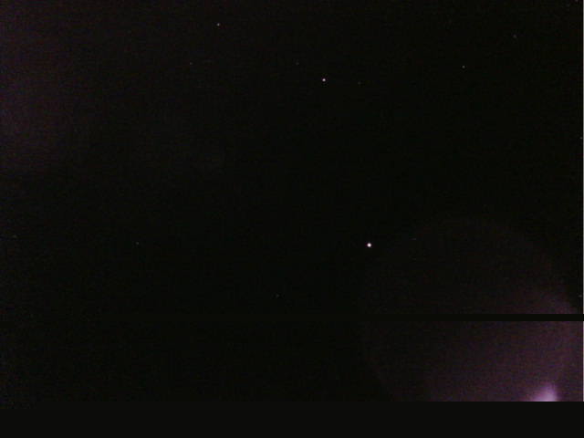
Besides this, it is also interesting to try to get the Moon in the image, as it has been done in other occasions. This not only gives a more interesting picture, but also helps the camera auto-exposure algorithm by providing a large bright object in the field of view. Past attempts to image the Earth alone have all yielded over-exposed images. It turns out that the orbit of DSLWP-B is ideal to image the eclipse, partly by chance and partly because of the nominal satellite attitude.
Recall that the camera of DSLWP-B is always pointing away from the Sun, because the satellite aims its solar panel towards the Sun. Since DSLWP-B orbits the Moon, this means that the Earth will be in the centre of the camera field of view whenever a solar eclipse happens. However, the satellite could be at any point of its orbit. It might happen that the Moon is between the satellite and the Earth, hiding the view, or, more likely, that the Moon is outside of the field of view of the camera.
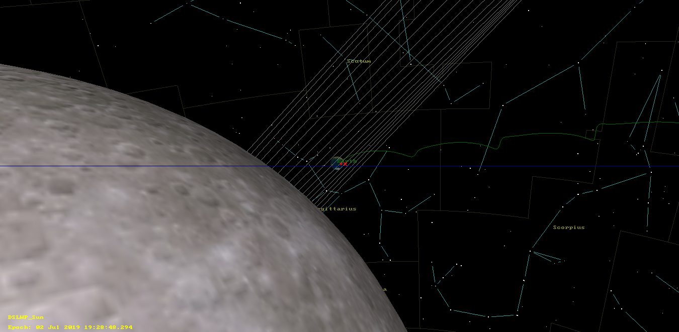
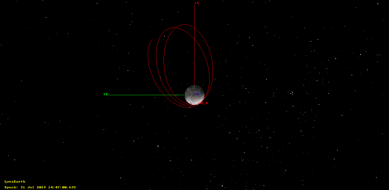
The total eclipse is observable between 18:01 and 20:45 UTC, with the maximum happening at 19:23. The two figures below show the positions of the Moon and Earth within the field of view of the camera. As explained above, the Earth is near the centre of the image during the eclipse. In the bottom figure we see that the Earth is hidden by the Moon until 19:27.

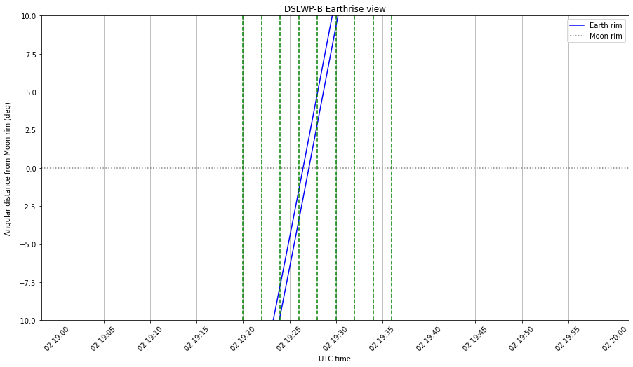
Therefore, it seems that this is an optimal chance to image the eclipse. The Earth will emerge behind the Moon very near to the eclipse maximum. Since DSLWP-B is orbiting at a lower altitude in comparison with other imaging sessions, the Moon will move rather quickly through the camera field of view and disappear in a matter of 10 minutes.
Thus, my recommendation is that instead of taking images every 10 minutes, as it has been done in other occasions, a smaller interval of 2 minutes is used instead. A series of 9 images starting at 19:20 is shown in the plot above as green lines. This gives good coverage of the eclipse and the Earth appearing behind the Moon.
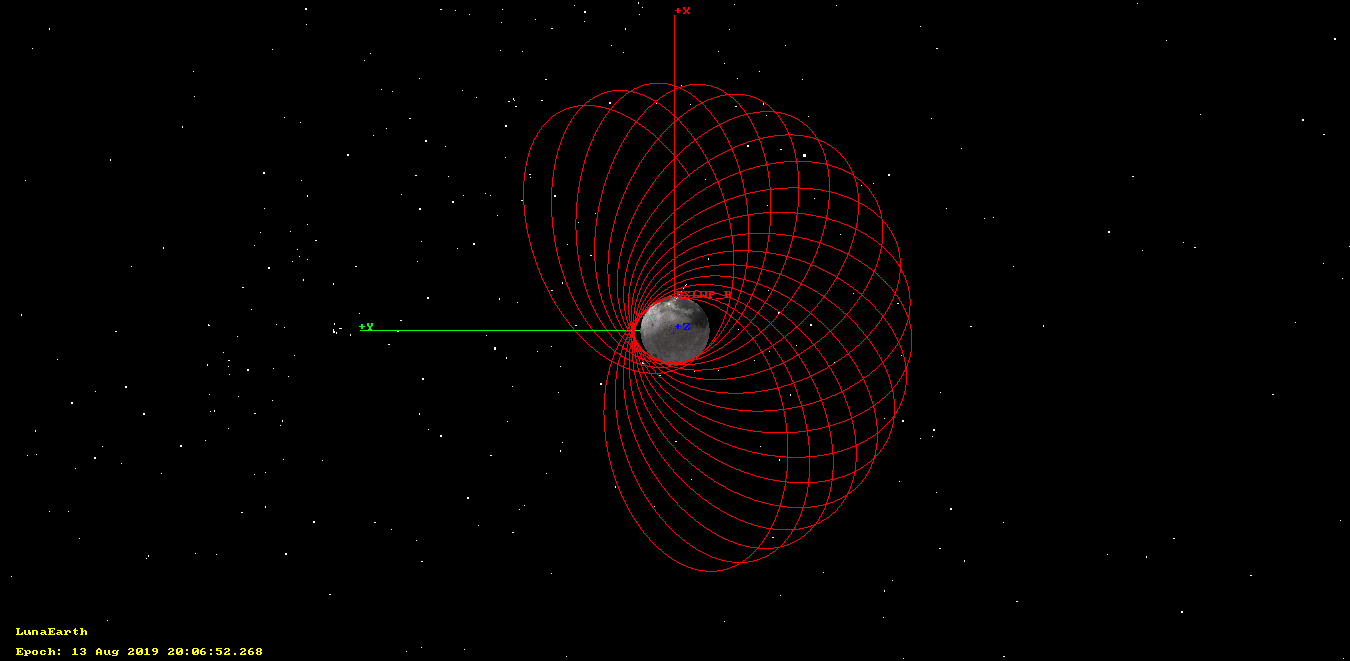
The figure below shows the simulation of the view in GMAT. Note that the field of view of the camera is smaller than what this image shows.