At the beginning of this week, JUICE, an ESA spacecraft that was launched in April 2023 and that will explore Jupiter’s icy moon, completed its lunar-Earth flyby. This is the first time that such a manoeuvre has been done. I’m far from an expert in orbital dynamics, but I hear that by doing a combined lunar-Earth flyby instead of the more traditional Earth flyby there can be delta-V savings for the mission. The IAC paper Improved interplanetary transfers with Lunar-Earth gravity assists seems to be the first that presented this idea, but I haven’t found the paper itself. The JUICE mission analysis report (CReMA) contains some more information, but it is not too detailed and somewhat outdated. Perhaps a good source to learn about this is a master’s thesis called Automatic extension of Earth and Earth-Moon resonant flybys, although I’ve only had time to read a small part of it.
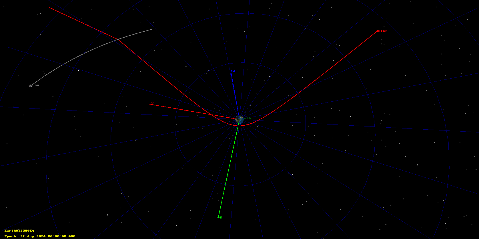
The following image that I made in GMAT with the mission SPICE kernels illustrates the geometry of the flybys. The lunar flyby happened on 2024-08-19 21:15 UTC, and the Earth flyby happened on 2024-08-20 21:56 UTC.
The Earth flyby happened 6840 km above the north Pacific ocean, so the spacecraft was visible from the Allen Telescope Array, in northern California, starting some minutes after the flyby. I thus decided to observe JUICE with one of the 6.1 m dishes of the array and record its X-band telemetry signal roughly between 22:00 and 23:00 UTC. That would be a fun way of “saying hello” again to the spacecraft (see the post where I recorded and decoded its telemetry when it launched in April last year).
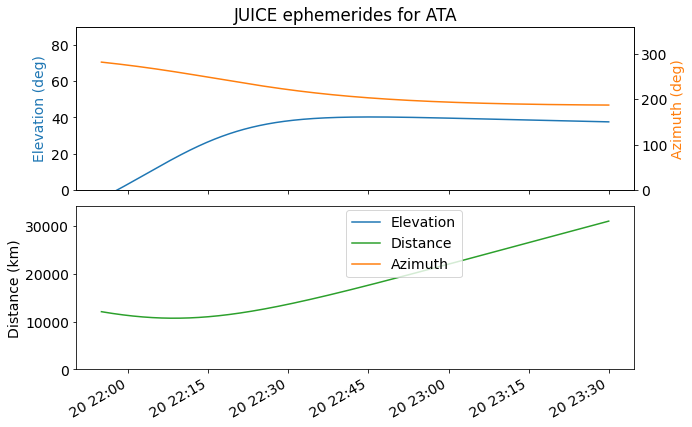
I prepared a tracking file for antenna pointing in the same way that I did for the OSIRIS-REx flyby during its sample capsule return. I used the SPICE kernels to compute a time series of azimuth and elevations for the antenna. For the spacecraft orbit I used the juice_orbc_000071_230414_310721_v01.bsp SPICE kernel, which was the latest available at the time. This kernel was created on 2024-08-15. The following plot shows the antenna azimuth and elevation and the distance to the spacecraft.
When I was about to begin observing, I saw a tweet from ESA Operations. Strangely the tweet has now been deleted. I hate it when information I once saw suddenly vanishes out of existence. I have the link to the tweet, but not a copy of it. It roughly said something along the lines of: “since JUICE is prepared for the cold thermal environment of Jupiter, to prevent it from overheating during the Earth flyby, data will not be transmitted to Earth until 2024-08-21 04:30 UTC”.
A problem with outreach communications is that they’re often vague with the hopes of simplifying to reach a wider audience. In this case, the context for the tweet was that ESA had run a livestream during the lunar flyby where they transmitted and showed images of the Moon in near-realtime. Postprocessed images with better quality were then released the next morning (see also this and related toots from Mark McCaughrean, who is one of the two persons responsible for the images). I think there was some word in social media that shortly after the Earth flyby some images would be shown, so the tweet served as a heads up that any images would need to wait until the next morning.
What wasn’t clear about the tweet is what this really meant about the spacecraft telemetry signal. Anyone familiar with spacecraft tracking will imagine that during the flyby there will be no groundstation coverage, because deep space stations can’t track that fast and probably won’t have the spacecraft in view. Therefore it’s clear that no images can be downloaded for some time around the flyby. But what about the telemetry signal? Does the tweet mean that there will be no housekeeping telemetry (which typically is sent all the time) either? Even no RF modulation at all? This might well be the case, especially since the tweet mentioned thermal reasons. If there isn’t going to be groundstation coverage for a while, why run the radio transmitter and generate more heat? But the way that the tweet was worded still made me doubt (I think the literal words were “it won’t transmit any more data”, but I don’t have the full sentence).
So after seeing that I wasn’t receiving any signal with the Allen Telescope Array, I wasn’t too surprised. I tweeted about this, as a quote tweet (repost) of the ESA Operations tweet.
I finished recording data at 22:30 UTC, since by then I was convinced that the transmitter was off and there was no point in continuing to record. I ran some additional tests to rule out a problem with the receiver. Unfortunately there were no good deep space X-band satellites in view at that time, since Mars was just setting. I tried with Parker Solar Probe, which was being tracked by Goldstone, but I didn’t know its frequency and didn’t have an estimate for how strong the signal should be. I didn’t see the signal. I also tried with ACE, which transmits at S-band and was also tracked by Goldstone. I could receive it just fine, so I don’t have much reason to suspect about the receiver.
Another potential reason why no signal could be detected is if there was an error in the ephemerides that caused a large enough antenna pointing error. I don’t think this was the case, even though the ephemerides were not updated after the lunar flyby. To make sure, I will rerun the pointing calculations with the next SPICE kernel that gets published and compare them. Pointing error is also the reason that I kept recording until 22:30 UTC. The effect of ephemerides error in pointing error would become smaller as the distance to the spacecraft increased with time.
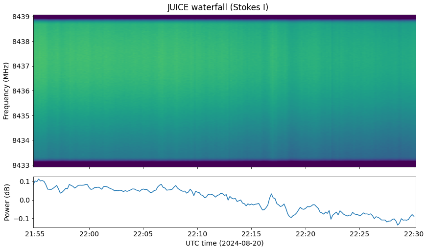
Just in case there was a faint signal, I have processed the recording to compute a waterfall with a resolution of 93.75 Hz and 10 seconds. The following two plots definitely show that there is no signal.
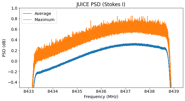
So with this, I finish the post as a failed observation of JUICE. I’ve decided do this write up because I think that, in science, negative results can be as important as positive results. In this case, the observation provides good evidence (especially now that the ESA Operations tweet is misteriously gone) that JUICE had the RF transmitter turned off during the Earth flyby. This is nothing transcendental, but rather an interesting tidbit of spacecraft operations trivia. The lack to detect any signals also reminds me of many astronomical observations, particularly those done as a followup to some transient, where if no signal is detected, the conclusion is often stated as “we establish upper bounds for the flux radiated by this source”.
To close with something more positive, I’ll mention that Alan Antoine F4LAU had a much more successful time tracking the lunar flyby with the AMSAT-DL 20 m antenna at Bochum Observatory, and he even found and decoded many images transmitted in the telemetry.
The materials used in this post can be found in this repository.