In my previous post I spoke about the recording of the telemetry signal from the Psyche spacecraft that I made just a few hours after launch with the Allen Telescope Array. In that post I analysed the physical aspects of the signal and the modulation and coding, but left the analysis of the telemetry frames for another post. That is the topic of this post. It will be a rather long and in-depth look at the telemetry, since I have managed to make sense of much of the structure of the data and there are several protocol layers to cover.
As a reminder from the previous post, the recording was around four hours long. During most of the first three hours, the spacecraft was slowly rotating around one of its axes, so the signal was only visible when the low-gain antenna pointed towards Earth. It was transmitting a low-rate 2 kbps signal. At some point it stopped rotating and switched to a higher rate 61.1 kbps signal. We will see important changes in the telemetry when this switch happens. Even though the high-rate signal represents only one quarter of the recording by duration, due to its 30x higher data rate, it represents most of the received telemetry by size.
AOS frames
The telemetry frames are CCSDS AOS frames. The spacecraft ID is 0xff. Interestingly, Psyche does not appeared in the SANA registry. However, the NAIF ID for Psyche is -255 (0xff is 255 in hex). Virtual channels 0, 1, and 63 (the only idle data virtual channel) are in use. Virtual channel 1 is only used with the high-rate signal. There is no operational control field. The frames contain a frame error control field (CRC-16), as is usual for Turbo coded frames. This was checked by the GNU Radio flowgraph that I used for decoding.
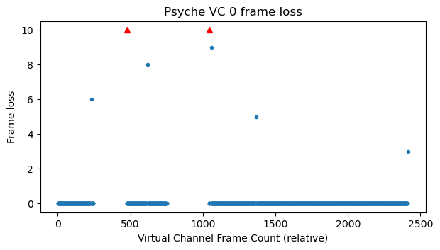
The following figures show the frame loss in each of the virtual channels. More than 10 lost frames in sequence are represented with a red arrow. In virtual channel 0 we can see large gaps when the spacecraft signal disappears because it is pointing away from the Earth. Besides these events, some of the frame losses are caused by uplink sweeps, since the PLL in the decoder I am using is not fast enough to track the sweep. As we will see below, virtual channel 0 is transmitted more or less at the same rate (in terms of frames per second) with the low rate signal and with the high-rate signal.
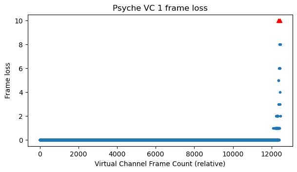
Virtual channel 1 starts transmitting data only at around 19:00 UTC, once the spacecraft has switched to high data rate. The frame loss corresponds to the spacecraft signal fading away as it sets below the elevation mask of the ATA.
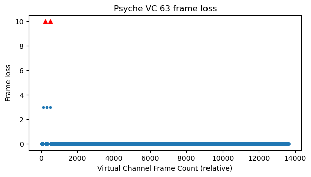
Virtual channel 63 stops being transmitted when VC 1 starts, but before this, a large number of VC 63 frames are transmitted in the high-rate signal. This explains why the gaps due to the spacecraft rotation appear at the very beginning of the plot and are very narrow compared to the plot for VC 0.
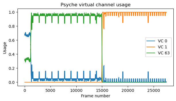
The relative virtual channel usage is shown next. With the low rate signal, VC 0 occupies 70% of the bandwidth, and the remaining 30% is taken up by VC 63. Once the high-rate signal starts, VC 0 continues transmitting at the same rate more or less. This represents now a very small fraction of the bandwidth, so most of the usage goes to VC 63. At some point, VC 1 starts transmitting data, taking up all the bandwidth that is left free by VC 0. The idle channel VC 63 disappears completely. There is also a small decrease in the data rate of VC 0 when this happens. Below we will examine the contents of VC 1 and see why it makes sense that it uses up all the spare bandwidth.
Virtual channel 0
Virtual channel 0 is used to transmit real-time telemetry. It contains CCSDS Space Packets using M_PDU. All the packets except for idle packets (APID 2047) have a secondary header. The secondary header contains a 6-byte timestamp that counts the number of \(2^{-16}\) second units elapsed since the J2000 epoch, 2000-01-01T00:00:00. As usual, more information about the spacecraft clock can be found in the SCLK kernels. These indicate that the epoch is supposed to be J2000 TDB rather than UTC, so there is an offset of about a minute with respect to UTC.
The idle packets in APID 2047 have a valid sequence count, but no secondary header. Their payload contains the starting fragment of an Easter egg ASCII text, which will be described below when I speak about virtual channel 63.
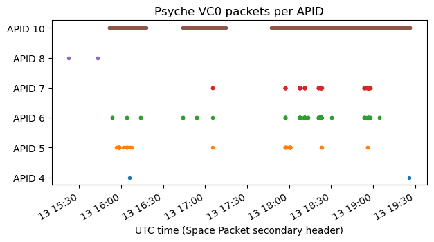
The non-idle APIDs are 4, 5, 6, 7, 8, and 10. Most of the data is transmitted in APID 10. The other APIDs are only used occasionally, as shown in this plot. Note that the timestamps for the APID 8 packets are not real time. These are recorded packets.
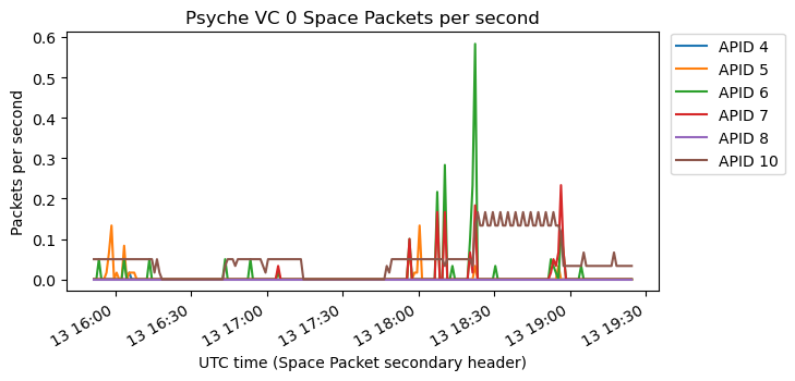
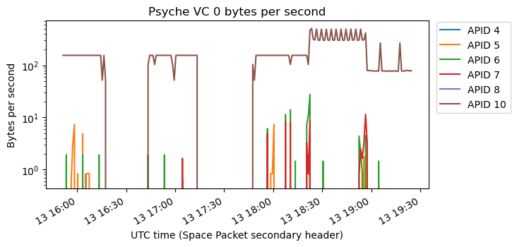
The next figures show the rate at which packets in each of the APIDs are transmitted. APID 10 is transmitted steadily, though we can see three different rates: one corresponding to the low-rate signal, another corresponding to the first half of the high-rate signal, until 19:00 UTC (when VC 1 starts), and another corresponding to the second half of the high-rate signal. The remaining APIDs are transmitted on demand as certain events happen.
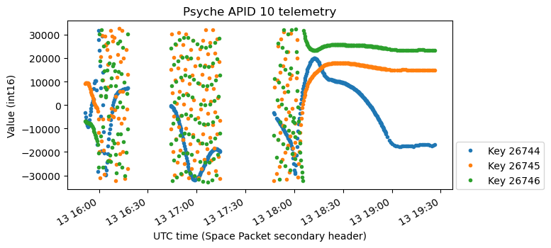
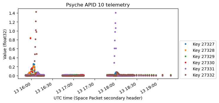
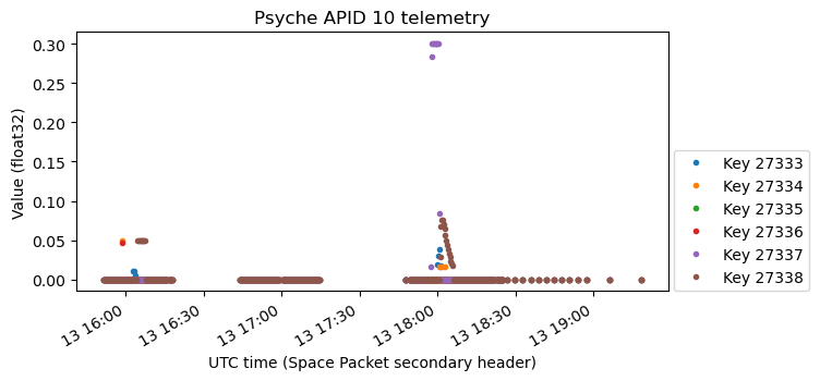
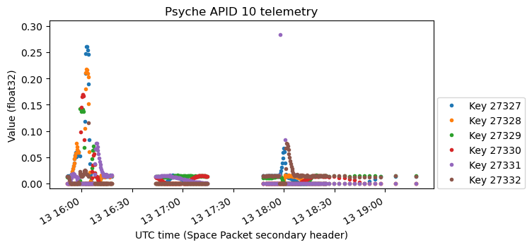
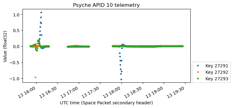
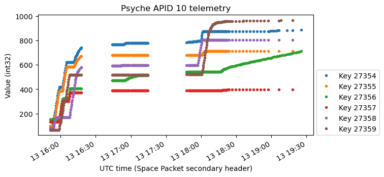
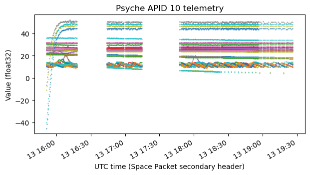
Here is a raster map for APID 10, which is perhaps the most interesting. There are plots for the other APIDs in the Jupyter notebook.
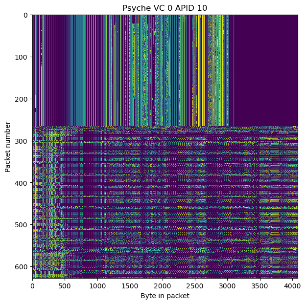
As we will see below, APID 10 is structured using key-value format. The first part of the data corresponds to the low-rate signal. In this part the same key-value pairs are transmitted in each packet, so the data lines up nicely. When the high-rate signal starts, more key-value pairs are activated, and so the data for a measurement no longer fits in a single packet (Psyche seems to use Space Packets of at most 4096 bytes). The key-value pairs overflow to the next Space Packets, and so the packet sizes are now different and the fields do not line up.
APIDs 4, 5, 6, 7 and 8
The Space Packets in these APIDs contain “sentences” (for lack of a better term) which start by a 6 character ASCII tag that seems to identify a spacecraft subsystem or function. Generally, the packets in each APID have different lengths. APIDs 4 and 8 only contain 2 packets each, with the tag GNC_16.
APID 5 contains many packets with the tag GNC_16. There are also a few packets with the tags EXE_16, DWN_16, and NVM_16. One of the DWN_16 sentences ends with the ASCII string ./eng/eha_selcrit_launch_safe_mode_recovery_60k. The timestamp of this packet is 18:23:09 UTC. This happens more or less at the same time that the high-data rate is enabled, so it seems related, specially because of the 60k (the data rate is 61.1 kbps, although this may be a coincidence).
APID 6 contains packets with the tags DWN_16, UPL_16, NVM_16 and EXE_16. In these packets there are several ASCII strings for what seem to be pre-stored command sequences. These are the following (each appears in several packets):
/eng/seq/stop_rotisserie.rel
/eng/seq/clt_24hrs.rel
/eng/seq/sdst_prime_ranging_on.rel
/eng/seq/set_dl_rate_60k_selcrit.rel
/eng/seq/set_dl_rate.mod
./eng/seq/repriortize_launch_dps_and_enable.rel
Most of these strings are in UPL_16, but sometimes the same string appears afterwards in an NVM_16 packet. I think that UPL stands for “uplink”, and these sentences are reports of telecommands received on the uplink that execute or set a pre-store sequence. NVM perhaps means non-volatile memory, and would indicate that some of these commands are written to non-volatile memory. Probably DWN means downlink, but these sentences do not contain any ASCII strings.
The stop_rotisserie refers to stopping the spacecraft rotisserie mode, in which the spacecraft points its solar panels to the sun and rotates slowly so that at certain times the low-gain antenna points towards Earth (more on this when we look at ADCS data below). This is something that I treated in the previous post. The sdst_prime_ranging_on refers to switching on the ranging transponder (SDST means Small Deep Space Transponder, which is the radio carried by Psyche). We also saw this happening in the previous post. Finally, set_dl_rate (and again, the 60k) refer to enabling the high-rate 61.1 kbps mode.
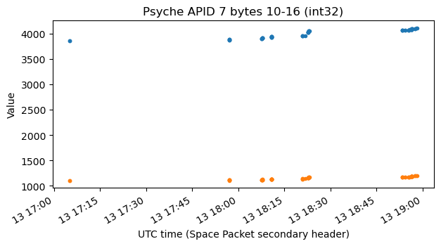
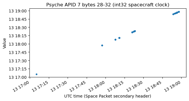
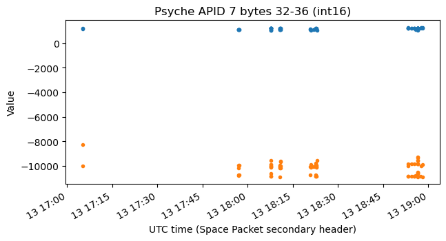
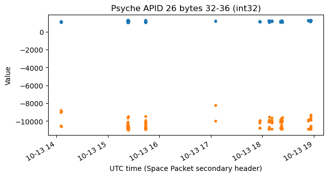
All the packets in APID 7 have the same size and start with the tag UPL_16. Looking at the raster map, it is apparent that the data in these packets is organized in fields of fixed size.
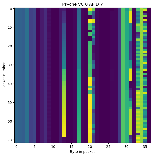
Here I have plotted the values of some of the fields in APID 7. I have no idea of what they represent, and I am not even certain that I am parsing them with the correct format, except for the int32 spacecraft timestamps, whose interpretation is clear. I suspect that these may be related to uplink signal radiometry, such as carrier frequency error and SNR, but I don’t have much arguments that support this.
APID 10
This APID contains real-time telemetry using a key-value format. Similarly to OSIRIS-REx, the keys have 16 bits, and the values have either 1, 2, 4 or 8 bytes. The size of each field is implicitly determined by its key. When analysing this APID, at first I was looking only at the low-rate data, where the fields line up nicely. I made a lot of plots using the offsets within the packet corresponding to each field. When I took a look at the high-rate data I saw that the fields became misaligned and this broke my plots, so I had to reverse-engineer all the value lengths and parse the key-value data properly as I did for OSIRIS-REx. This took some work, but luckily much less than for OSIRIS-REx. There were “only” 4748 different keys to go through. Of these, only 553 appear in the low-rate data.
The plots that I have for this APID correspond to the fields that I identified as interesting when looking at the low-rate data only. I have not gone through the contents of the 4195 keys that only appear in the high-rate data to see what is there. There are many plots in the Jupyter notebook. Here I will only include a selection.
The most interesting data in APID 10 is maybe the ADCS data, so let’s start with that.
ADCS telemetry: attitude quaternions
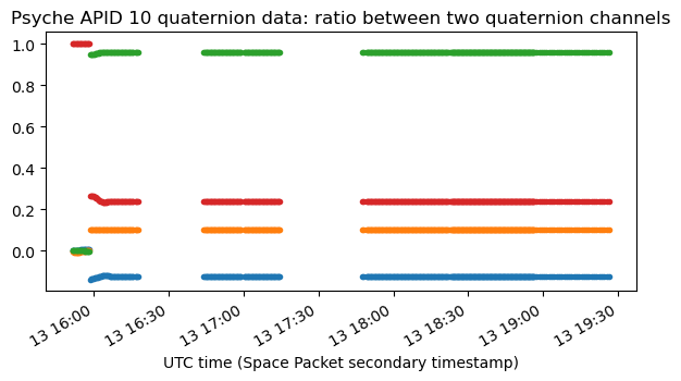
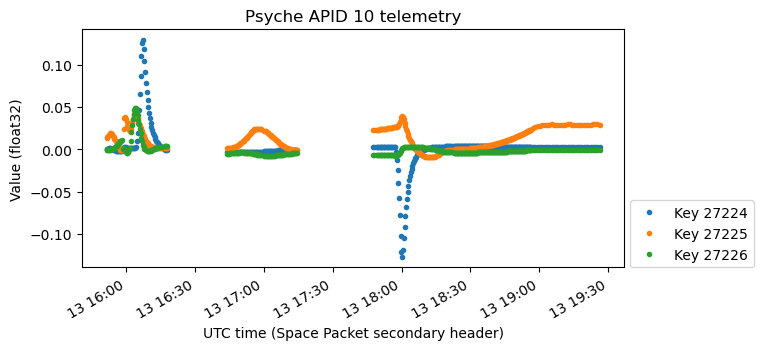
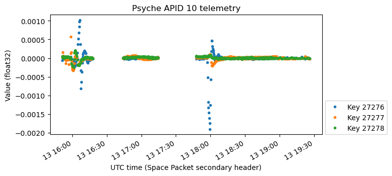
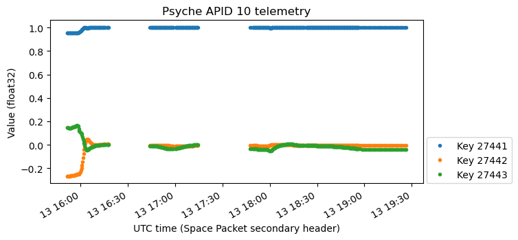
There are two groups of telemetry variables that contain quaternion data (which is easy to spot because the sum of squares of the four components is one). These are shown here.
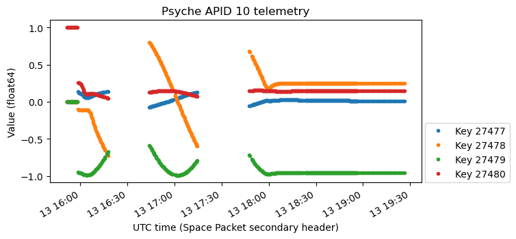
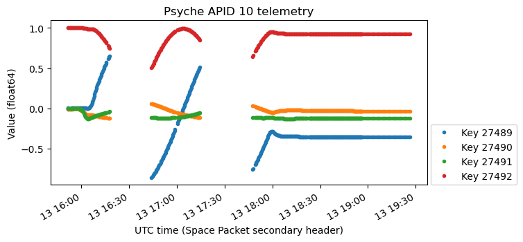
Already looking at these plots we can see that they describe some form of slow rotation that stops at 18:00 UTC. The two plots start with the same value: a one in the last component, and zero in the rest. These quaternions are in scalar-last format, because as we will see, interpreting them as such gives meaningful results. Therefore, this initial value corresponds to the quaternion 1, which represents no rotation (the identity function). This is a reasonable “reset value”.
One important difference between the two plots is that the first has a jump. The data starts at 1 constantly until at some it snaps to a new value and starts moving. On the other hand, the second plot is continuous. The data moves in a similar way in both plots, but there is no jump on the second plot.
Let us now do the usual math to explore these quaternions further, starting with the first plot. We denote by \(q(t)\) the quaternion at time \(t\). We compute \(h(t) = q(t)^{-1} q(t_0)\) for a suitable choice of a reference time \(t_0\) and plot the axis of rotation of the quaternion \(h(t)\) (which is the imaginary part of the quaternion normalized to unit norm). This gives the following plot. The reference time \(t_0\) is indicated with a vertical grey line.
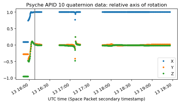
We see that after \(t_0\) the quaternion \(h(t)\) describes a rotation about the X axis. Having the spacecraft be rotating all the time about its X axis is a reasonable thing, so this confirms that \(q(t)\) is the quaternion representing the rotation from the spacecraft body frame to a certain inertial frame. The quaternion \(h(t)\) corresponds to the relative rotation of the spacecraft between time \(t_0\) and time \(t\), expressed in body coordinates. I have chosen the time \(t_0\) when the spacecraft starts the rotisserie mode, which consists in rotating about the X body axis.
The astute reader might have spotted that there is something going on at around 17:10 UTC. However, what happens here is simply that the spacecraft has completed exactly a full rotation since \(t_0\). Therefore \(h(t)\) is close to 1 and determining the axis of rotation is ill-conditioned.
We now compute and plot the angle of the rotation \(h(t)\). We see that the rotation has a constant angular rate from around 16:00 to 18:00 UTC, and then it stops.
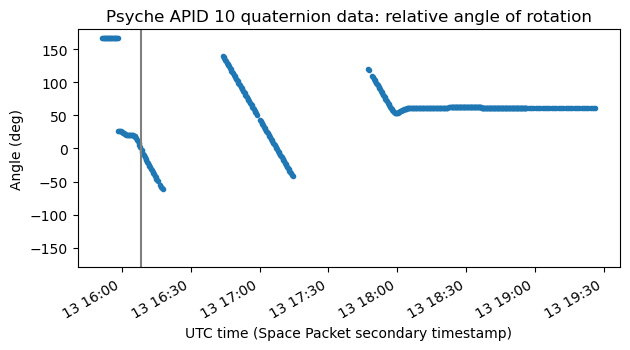
From the above plot we can measure the rotation rate. It is almost exactly -0.1 deg/s. This means that a full rotation takes exactly one hour. This is the rotisserie mode. The spacecraft is rotating about its X axis at a rate of one rotation per hour.
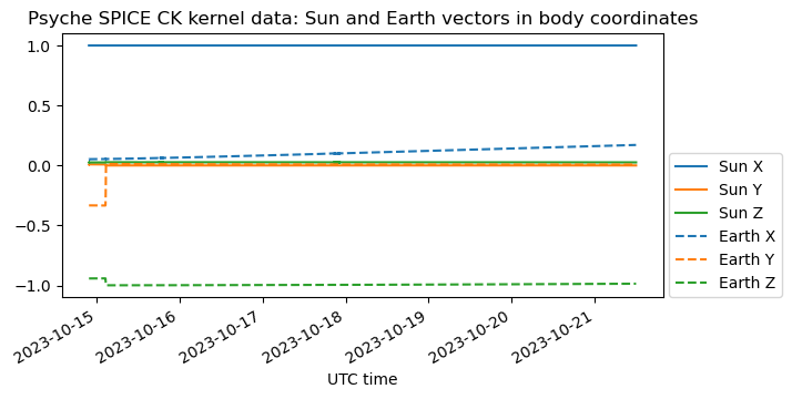
Now let us try to verify the inertial frame for these quaternions. Typically it will be the J2000 equatorial system or the ICRF system (and these two are close enough that we cannot tell the difference based on the telemetry data). To do this, we compute the Sun vector as seen by the spacecraft. I have used SPICE kernels and SpiceyPy for this, since I will also be doing some other SPICE calculations, but a heliocentric state vector obtained from HORIZONS would suffice.
We use the body to intertial quaternions \(q(t)\) to find the inertial orientation of the spacecraft X body axis. This can be computed as the imaginary part of \(q(t)iq(t)^{-1}\). The plot below compares this inertial vector with the Sun vector. We see that the two are very similar. This confirms that the intertial reference used for the quaterions is J2000 (or ICRF), and that the spacecraft is pointing its X axis towards the Sun (except at around 15:50 UTC, when it is finishing to point itself towards the Sun).
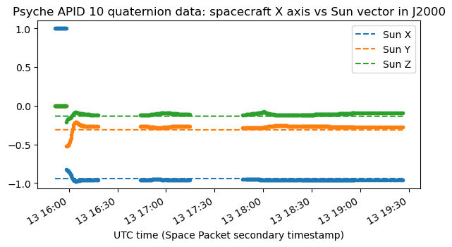
We know that in the rotisserie mode one of the spacecraft axes perpendicular to the solar panels axis is pointed towards the Sun and the spacecraft slowly rotates about this axis to try to find Earth with its low-gain antenna. The solar panels can rotate about their axis, so in this way they can be pointed towards the Sun all the time for maximum illumination while the spacecraft tries to communicate with Earth. In the quaternion data, the axis that is pointed towards the Sun is the X axis.
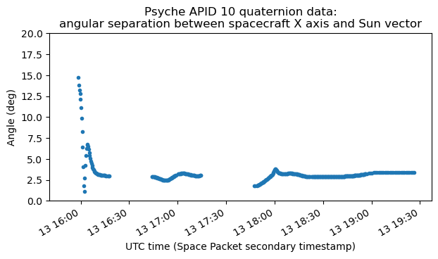
It is also interesting to plot the angular separation between the spacecraft X axis and the Sun vector. We see that there is a pointing error of a couple degrees, and that at the beginning of the observation with the ATA the spacecraft was still off-pointing from the Sun by about 15 degrees.
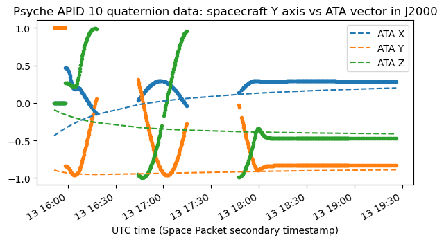
Now we do the same exercise with the Earth vector seen from the spacecraft. This will give us information about the location of the low-gain antenna in the spacecraft body, according to the time intervals when we saw the signal disappear. Since at the beginning of the observation the spacecraft is still quite near Earth, instead of using the Earth vector, I have used the vector joining the spacecraft and the ATA, as this would indicate better what we see from the ATA.
By looking at what happens with each of the spacecraft body axes, it turns out that the Y axis is quite close to the ATA vector when the spacecraft stops rotating at 18:00 UTC. Then the spacecraft was communicating with the DSN station at Goldstone, which is near enough the ATA that the distinction doesn’t matter.
The situation is understood more clearly by looking at the angular separation between the spacecraft Y axis and the ATA vector. We not only see that the rotation stops at 18:00 UTC when the angle is close to zero, but also that the periods when we see the spacecraft signal (and so have telemetry data to plot) are those when the angular error is roughly less than 90 degrees.
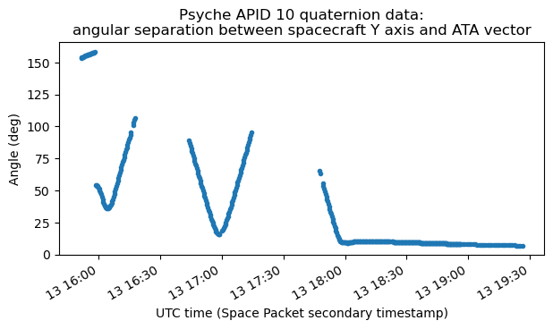
This makes a lot of sense. It means that the spacecraft low-gain antenna that is active is located on the +Y face of the spacecraft, and has roughly hemispherical coverage. When the off-boresight angle is smaller than 90 degrees we can receive the signal. When it grows larger than 90 degrees, the spacecraft body gets in the way and we lose the signal. I don’t know why the critical angles at which the signal appears and disappears are not consistent in each rotation (in particular, in the last partial rotation the signal only appears at a 75 deg angle). Maybe the reason is simply that free-space path loss is increasing significantly as the spacecraft gets away from Earth, so each time we need more antenna gain to be able to see the signal.
This explanation of the ADCS quaternions looks quite satisfactory, but now we can read the spacecraft frame kernels to learn more about how the spacecraft axes are defined and where each element is placed. According to the SPICE kernels, the solar panels are along the Y axis. The high-gain antenna points towards the +Z axis (with an offset of 10 degrees). There are low-gain antennas in the -Z, +X and -X faces. However this is not consistent with what we have seen in the ADCS telemetry, for it appeared that the active low-gain antenna was in the +Y face.
Looking in more detail at the frame kernels, we see that in version 0.4 there was an update in the low-gain antenna frames:
Renamed LGA frames from PSYC_LGA_PZ, PSYC_LGA_PY, and PSYC_LGA_MY to PSYC_LGA_MZ, PSYC_LGA_PX, and PSYC_LGA_MX and changed their alignments accordingly (see [7]).
Unfortunately, reference [7] does not seem to be publicly available. I’m interpreting this to mean that the spacecraft body axes were redefined rather than the positions of the low-gain antennas being moved around (specially because there are not many places to put them: since it does not make sense to put an LGA on the faces occupied by the HGA and the solar panels, there are only three free faces to put three LGAs). Using this information we can make a table that relates the frame of kernel v0.4 and later, the frame of kernel v0.3 and earlier, and the frame used in the ADCS telemetry. Surprisingly, the three are different. They are all right-handed systems, which is a good sanity check. The difference between kernels v0.4 and v0.3 is simply a swap in X and Y, with the required sign change of Z to preserve the orientation. The ADCS telemetry frame uses the same X axis as kernel v0.4, but the Z and Y axes are swapped (with a sign flip, to preserve the orientation).
| ADCS telemetry | Kernel v0.4 | Kernel v0.3 |
|---|---|---|
| X | X | Y |
| Z | Y | X |
| -Y | Z | -Z |
Since it seems weird that the ADCS telemetry uses a different frame compared to the SPICE kernels, I wanted to make sure that this wasn’t due to an error on my side. To this end, I have compared the SPICE CK kernels that contain the attitude of the spacecraft with the ADCS telemetry. Unfortunately there is no data for 2023-10-13, which is the day when the spacecraft was launched. The data in the NAIF repository starts on 2023-10-14 (there is some data from 2023-10-13, but it is for the solar panels rotation with respect to the spacecraft body, not for the spacecraft body rotation with respect to J2000). Even so, plotting the data after 2023-10-14 the situation is clear: the spacecraft is always pointing its +X face to the Sun and its -Z face to the Earth (except for a small deviation before 2023-10-15). If we assume that the same attitude was used on 2023-10-13 after 18:00 UTC, then this confirms that the ADCS telemetry Y axis is the same as the SPICE kernel -Z axis.
To sum up, the spacecraft solar panels are along a certain axis (Z in the ADCS telemetry), and can rotate about this axis. On one of the remaining four faces there is the high-gain antenna (-Y in the ADCS telemetry), and on each of the other three faces there is a low-gain antenna (+X, -X and +Y in the ADCS telemetry). In the rotisserie mode the spacecraft points its +X face towards the Sun, so that the solar panels can be illuminated maximally, and starts rotating about the X axis at a rate of one rotation per hour.
The Sun and Earth are roughly at a 90 degrees angle as seen from the spacecraft. This is the case for almost any spacecraft launching from Earth into deep space, since its velocity vector with respect to the Sun would be nearly parallel to Earth’s velocity vector, but of a different magnitude, so the relative velocity between the spacecraft and Earth is also nearly parallel to the Earth’s velocity vector with respect to the Sun, and hence orthogonal to the vector joining the Earth and the Sun. Therefore, the +Y, -Y, +Z and -Z faces take turns pointing towards the Earth. Of these faces, there is only a low-gain antenna in the +Y face. The +Z and -Z faces are taken up by the solar panels, and -Y by the high-gain antenna (all this using the ADCS telemetry frame). In consequence, the low-gain antenna in the +Y face is the one that needs to be used for the initial signal acquisition.
I think that all this procedure is done in a very simple way for maximum reliability. The spacecraft can keep pointing to the Sun by using Sun sensors on the +X face. The solar panels can be oriented with a fixed rotation with respect to the spacecraft body: the one that points them in the direction of the +X face. Then the spacecraft simply rotates about the X axis at constant rate. On ground they measure when the low-gain antenna is pointing to Earth by taking note of when the signal appears and disappears, and then they simply telecommand the spacecraft to stop rotating when they know that the low-gain antenna is again pointing directly to Earth. This procedure can be executed even if the ADCS system is not working correctly and the spacecraft doesn’t know its absolute orientation in space (even though in this case looking at the telemetry we see that the spacecraft knew its orientation).
Let us now look at the second attitude quaternion plot. To study this, we denote by \(q_2(t)\) the quaternion for time \(t\) corresponding to the second plot. We compute and plot \(q_2(t) q(t)^{-1}\). Except at the beginning, this gives a constant result.
This basically means that \(q_2(t)\) also describes the body to inertial rotation, but using a different inertial system. The rotation from J2000 to this other inertial system is given by the constant quaternion of the above plot. However, this new inertial system does not seem to be any meaningful system. I think that even though mathematically correct, this is not a good way of thinking about the situation.
If we remember that the quaternions \(q_2(t)\) start with the value 1 and are continuous, then the conclusion is that they represent the rotation from the body coordinates to inertial coordinates relative to the inertial orientation that the spacecraft had when the ADCS was first started. As such, it seems a form of dead-reckoning system that doesn’t attempt to solve the absolute orientation in space, but rather keeps track of orientation changes with respect to an initial orientation. This still does not explain why the plot above is changing slightly around 16:00 UTC. I think that this might be because the spacecraft was still smoothly solving for its absolute orientation, so the quaternions \(q(t)\) still do not represent the rotation from body to J2000 coordinates, but rather to a frame that is close to J2000 and smoothly and slowly gets aligned with it (this frame is the spacecraft’s “best knowledge” of J2000).
ADCS telemetry: gyroscopes
Now that we have studied the quaternion data, it is easier to locate and understand gyroscope data in the telemetry, because we know how the angular velocity should look like. Here is one set of gyroscope variables.
Between 16:10 and 18:00 UTC the X component shows a nonzero constant value, because the spacecraft is in rotisserie mode rotating about its X axis. The Y and Z components are zero as expected. After 18:00 UTC all the rotation stops. We can also see that at 16:00 UTC there is rotation in the three axes, because the spacecraft was rotating to point its +X face towards the Sun.
The value of the X component during the rotisserie rotation is 0.001745. This means that the units of this gyroscope data are radians/s. If we do the unit conversion to deg/s, we obtain 0.1 deg/s as expected.
Here is another set of gyroscope data. The units are also radians/s. Comparing to the plot above, this is noisier. I think that the previous plot corresponds to the set (commanded) angular velocity, and this one is measured angular velocity. In fact, the previous plot consists of perfectly straight line segments. In this plot we can see elements typical of a control system, such as some overshoot and ringing.
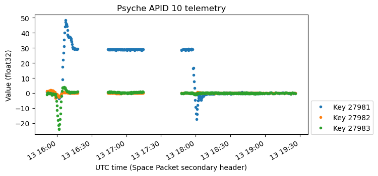
The next plot shows more gyroscope data. The sign of all the axes is inverted, and the scale is different. I have not figured out a reasonable scale factor for these values. The constant rotation at 0.1 deg/s has the value -28.936 here.
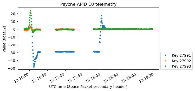
The following variables seem to have the same data but with opposite sign.
Other telemetry values related to the ADCS
Since the rotisserie mode is a characteristic event with definite start and stop times, it is possible to find other variables in the telemetry that are affected by the rotisserie rotation. Many of these are probably related to the ADCS, although it is more difficult to understand exactly how.
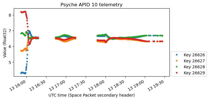
The first of these is the following. It is not at all clear to me what this means, but there is a notable change when the spacecraft points the +X axis towards the Sun. What I find most peculiar about these values is that they seem to be centred on 6.5.
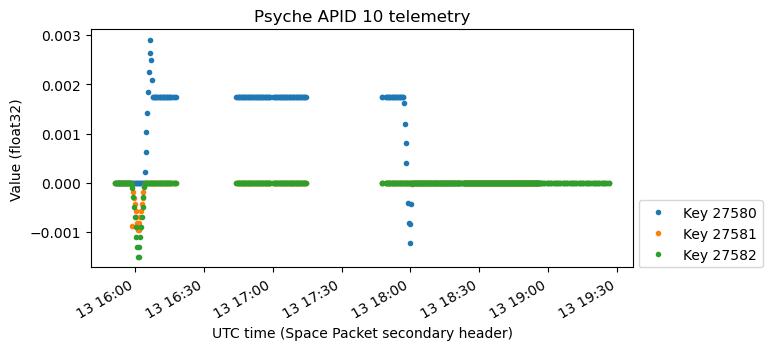
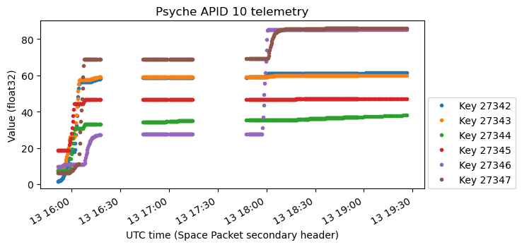
Here is another interesting set of variables. They seem to increment whenever there is angular acceleration. Interestingly, the change is always positive. If these variables showed somehow the integral of angular acceleration, we would expect changes of opposite sign when the rotisserie starts versus when it ends.
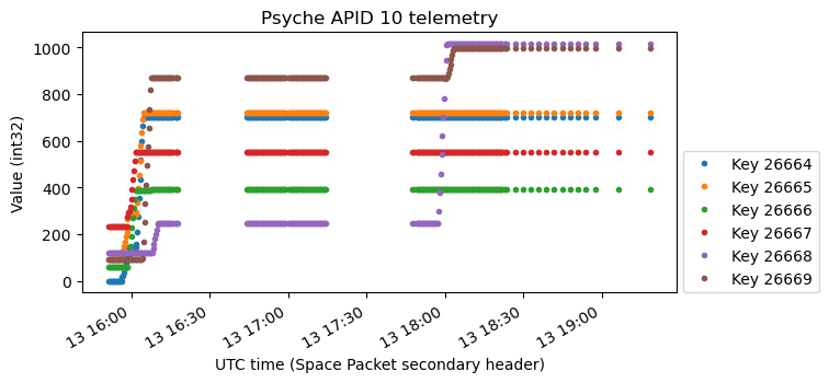
However, a closer look reveals that these variables come in pairs. The purple and brown seem to be the ones associated with the X axis. When the rotisserie starts (causing an angular acceleration in one direction), the brown variable increases a lot and the purple variable increases only slightly. When the rotisserie stops (causing an angular acceleration in the opposite direction), the behaviour is reversed: the purple variable increases a lot and the brown one only slightly. This means that we should actually look at the difference between the purple minus brown, and so on for the other channels.
I think that these variables represent the reaction wheels angular velocity. It seems that there are counteracting pairs of reaction wheels. To apply angular acceleration on an axis, the two counteracting pairs are spun up. One of them is spun up much more, to cause the net torque, and the other one is spun up only slightly. I’m not an expert on reaction wheels, so I don’t know why it would be advantageous to do it like this.
The next plot is also interesting. There are three int16 channels, and the values cover the full range. There appears to be aliasing in the measurements of Y and Z when the spacecraft is in rotisserie mode. The X value does not wrap around, except maybe at the beginning. I think these are angles of some sort, but they are “magnified”, in the sense that the full int16 range does not correspond to a full rotation, but only to a few degrees. This would explain why the slow rotisserie rotation is constantly causing the Y and Z angles to wrap around and alias.
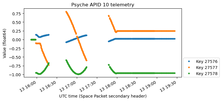
The next plot is much easier to explain. It is just the i, j, k values of the body to J2000 quaternions. The scalar part is missing, but this is easy to recover from the other components if we know that the quaternions have been normalized so that the scalar part is non-negative (which was the case in the plots of the previous section), because we know that the sum of squares of the four quaternion components must be one.
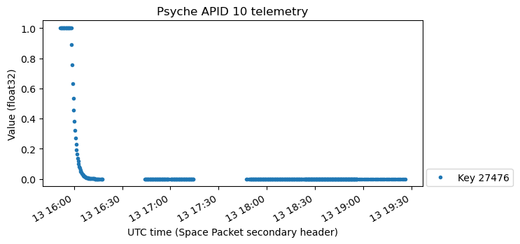
The next plot shows what appears to be an exponential decay from 1 to 0 that coincides with the spacecraft moving to point towards the Sun. I don’t know what this represents. Maybe it is not related to the ADCS, but to another subsystem. There are other plots similar to this one in the Jupyter notebook.
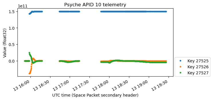
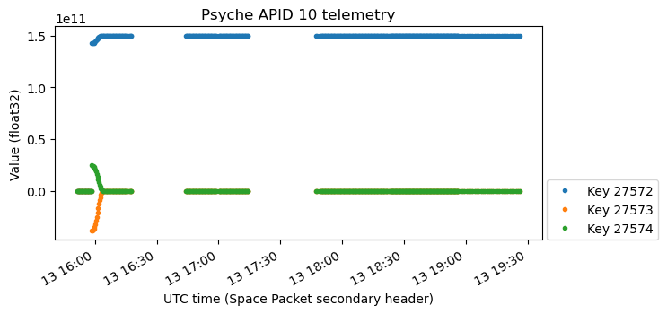
These three variables seem to be related to the spacecraft attitude, since we can see the movement of the spacecraft pointing towards the Sun. The scale is curious, because the X component has a value around \(1.5\cdot 10^{11}\). I think these variables are simply the vector joining the spacecraft and the Sun, in spacecraft body coordinates and metre units. An astronomical unit is approximately \(1.496\cdot 10^{11}\) metres, so this explanation makes sense.
The next value appears to be the time derivatives of what I identified as the reaction wheels angular velocities. This means that these values would represent the reaction wheels angular accelerations or torques. We can clearly see the start and end of the rotisserie, marked by large accelerations in the brown and purple channels respectively.
The next plot seems to be related to the one above, but I cannot explain why it looks like so. It seems that it only contain values as large as 0.30, with larger values going off-scale and showing up as zero, but this is not a complete explanation, because also some small values seem to be clamped down to zero, and some of the curves we would expect to see are missing.
For comparison, here is how the reaction wheels angular acceleration plot looks like if we only plot values smaller than 0.3.
Here is something that seems to show the total angular rate (irrespective of axis), but it is also strange because it has a second channel. Maybe what I have plotted as the second channel is an unrelated variable.
The next plot shows the angular acceleration in the spacecraft body axes. This one has the opposite signs we would expect for the beginning and end of the rotisserie.
Here are two other sets of variables that are probably related to angular acceleration. The first one is somewhat strange because the data on the Y and Z channels is not orders of magnitude smaller than the X channel, which is what we would expect.
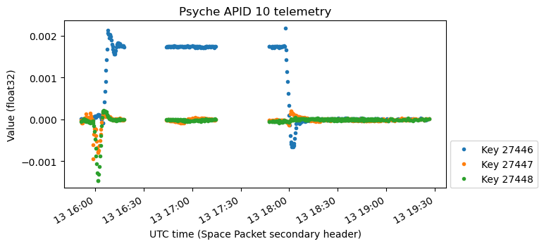
Next we have two plots related to the reaction wheels. The first plot looks very similar to the one we have shown above, but there are some small differences. The purple and brown channels settle smoothly after increasing by a small amount. The green channel keeps increasing slightly. Maybe the plot above corresponds to commanded values, since it seems to be formed by exact straight lines, and this one gives measured values.
The next plot is strange. The shape of the increments is qualitatively the same as in the plot above, but the magnitudes do not seem to make any sense. It looks as if a different non-linear scaling was applied to each channel to obtain this plot.
The next plot seems to be the normalized Sun vector in spacecraft body axes. Compare this to the plot above in which the X channel had a value of \(1.5\cdot 10^{11}\).
The following is also the Sun vector, this time in units of metres. However, compared to the plot above it looks too perfect. The Y and Z components stay exactly at zero. So probably this plot corresponds to the commanded value, and the plot above gives the measured value.
Other telemetry values
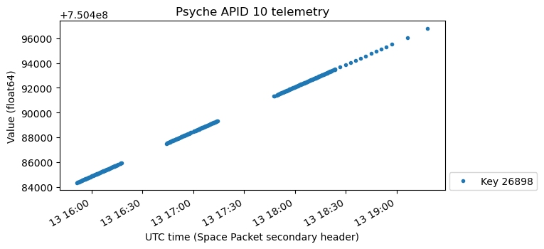
There are many keys that contain spacecraft timestamps, usually as a float64. These would be the timestamps for the data with neighbouring keys. However, the values corresponding to these keys are close to the timestamps on the Space Packet secondary header, so in all the plots I am using the secondary header for the x-axis, rather than trying to find the applicable timestamp keys for the data I’m plotting.
There are many variables with keys around 57400 that show similar behaviour and ranges. I think that all these are temperatures in Celsius. These variables are shown in the plot below. We can see that there is a group of variables that increases from around -40 to around 50 slightly before 16:00 UTC. There are many variables that have more or less constant values spread between 20 and 35. And there is another group of variables that show a sawtooth behaviour and range between 10 and 15. This last group would correspond to temperatures of components that are actively heated with an on-off controller.
There are other plots in the Jupyter notebook that I have not included here. If you browse through them, perhaps you have an idea as to what they might represent.
Virtual channel 1
Virtual channel 1 is used to send files using the CCSDS CFDP protocol. Version 0 of the protocol is used, although version 1 was released in 2020. Therefore, the applicable documentation is the historical CCSDS 727.0-B-4 instead of the current CCSDS 727.0-B-5.
The virtual channel 1 AOS frames carry CCSDS Space Packets using M_PDU. The following APIDs, in addition to the idle APID 2047, are in use during the observation I made with the ATA: 102, 103, 104, 107, 300, 318, 1002. As in virtual channel 0, all the Space Packets except for the idle ones have a secondary header with a 6-byte timestamp. The APID 2047 idle packets are constructed in the same way as for virtual channel 0.
The payload of each non-idle Space Packet has 4 bytes (which might be part of the secondary header, for all I know) followed by a CFDP PDU. These extra 4 bytes seem to be divided into two 2-byte fields. The first field has a constant value for all the packets of the same file, and sometimes the same value is repeated for several files. The second field is a counter that gives the sequence number of the packets of each file, resetting to zero when a new file starts.
The way in which each file is transmitted is always the same. First a metadata PDU is sent. This contains the length and name of the file. Then the file data blocks packets are transmitted. At the end, an EOF PDU is sent informing of the correct transmission and giving the file checksum. Transmission mode 1 (unacknowledged) is used. The following shows an example of the CFDP PDUs of one file transmitted in APID 1002. The PDUs are parsed with construct. The file is small enough that it fits into a single file data packet, but in other cases there are many data packets per file.
Container(
  header=Container(
    version=0, pdu_type=0, direction=0,
    transmission_mode=1, crc_flag=False,
    reserved=0, pdu_data_field_length=54,
    reserved2=0, length_of_entity_ids=0,
    reserved3=0,
    length_of_transaction_sequence_number=7,
    source_entity_id=255,
    transaction_sequence_number=3223303882434963412,
    destination_entity_id=1),
 file_directive_code=7,
 eof_pdu=None,
 metadata_pdu=Container(
  segmentation_control=1, reserved=0,
  length_of_file=126,
  source_file_name=Container(
    length=23, value=b'1002_0750483917-0670406'),
  destination_file_name=Container(
    length=23, value=b'1002_0750483917-0670406'),
 options=ListContainer([])),
 file_data=None)

Container(
  header=Container(
    version=0, pdu_type=1, direction=0,
    transmission_mode=1, crc_flag=False,
    reserved=0, pdu_data_field_length=130,
    reserved2=0, length_of_entity_ids=0,
    reserved3=0,
    length_of_transaction_sequence_number=7,
    source_entity_id=255,
    transaction_sequence_number=3223303882434963412,
    destination_entity_id=1),
 file_directive_code=None,
 eof_pdu=None, metadata_pdu=None,
 file_data=Container(
   offset=0,
   file_data=b',\xbby\x98\x11\xa7p'[...],
)

Container(
  header=Container(
    version=0, pdu_type=0, direction=0,
    transmission_mode=1, crc_flag=False,
    reserved=0, pdu_data_field_length=10,
    reserved2=0, length_of_entity_ids=0,
    reserved3=0,
    length_of_transaction_sequence_number=7,
    source_entity_id=255,
    transaction_sequence_number=3223303882434963412,
    destination_entity_id=1),
  file_directive_code=4,
  eof_pdu=Container(
    condition_code=uEnumIntegerString.new(0, 'NoError'),
    spare=0, file_checksum=1827264513,
    file_size=126, fault_location=None),
  metadata_pdu=None,
  file_data=None)
The transaction sequence numbers are a 64-bit integer. The 32 MSBs of these integers are the spacecraft timestamp in seconds corresponding to the file (file creation or similar). The 32 LSBs could be the sub-second part of the timestamp or something else.
The filenames always follow the same format: 1002_0750483917-0670406. First we have the APID where the file is transmitted, a _ separator, then the file timestamp in seconds (which is the same as the 32 MSBs of the transaction sequence number), a - separator, and finally a number that I have not figured out what it is. The same filename is used as source and destination filename.
All the Space Packets corresponding to a file have the same timestamp in the secondary header, which matches the timestamp used for the file name and transaction sequence number. Therefore, I do not have a good way of knowing when each Space Packet was actually transmitted, since I don’t have assigned reception timestamps to the AOS frames. The following plot shows the secondary header timestamp of each Space Packet, in the order in which they were received and coloured by APID. It gives a good idea of when each file is transmitted. The x-axis is simply a packet counter, but it roughly corresponds to time since virtual channel 1 became active.
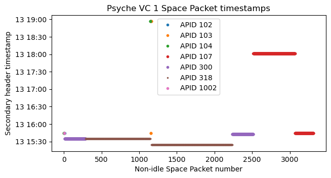
We see that only one file is transmitted at a time. There are some very short files in APIDs 102, 103 and 104, and longer files in APIDs 107, 300 and 318. When the observation finishes, a file from APID 107 is still being transmitted. Note that the timestamps of many of the files are before the beginning of the observation I did with the ATA. All these files contain recorded data. Their transmission only begins some time after 19:00 UTC.
Now this explains why when virtual channel 1 becomes active there are no more virtual channel 63 idle frames. The spacecraft is commanded to transmit a bunch of files as fast as possible, so all the bandwidth unused by virtual channel 0 for real-time telemetry is used by virtual channel 1 for file transmission. Transmitting all these files is a logical thing to do at this point. There was a lot of telemetry data that could not be received in real-time, both because the spacecraft was transmitting a low rate 2 kbps signal (so some data could not even be transmitted), and also because there were times when the signal was not visible because the antenna was pointing away from Earth. Transmitting the recorded telemetry over CFDP files now with the 61.1 kbps signal is the way to recover this missing data.
APIDs 102, 103, 104
The CFDP files sent in APIDs 102, 103 and 104 contain CCSDS Space Packets from APIDs 24, 25 and 26 respectively. The files are simply a concatenation of the Space Packets, with no extra headers or delimiters. The contents of these packets are very similar to the packets in APIDs 5, 6 and 7 that we saw in the real-time telemetry. I think that APIDs 24, 25, and 26 are simply the same kind of data, but recorded instead of real-time.
APID 102 has sent only two small files (with packets from APID 24). One of them contains four PLD_16 “sentences”, and the other one contains one GNC_16 sentence.
The packets from APID 25 contain sentences from DWN_16, EXE_16, NVM_16, and GNC_16. There are three DWN_16 sentences that contain ASCII strings. One of them is /eng/eha_selcrit_sys_sa_deploy. I guess this corresponds to the solar array deployment. The two other strings are /eng/eha_selcrit_sys_safe_cgs and /eng/eha_selcrit_launch_safe_mode_recovery_60k.
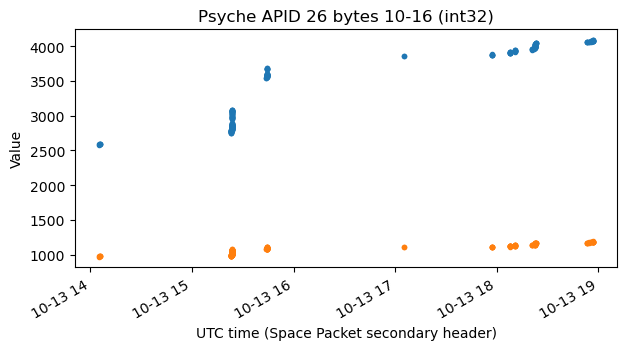
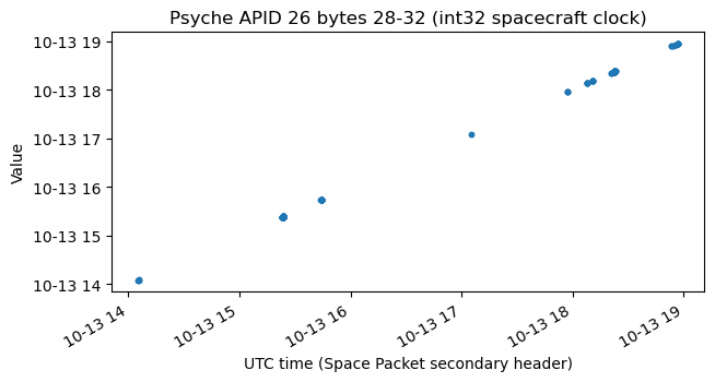
APID 26 contains sentences that begin by UPL_16 and have a fixed length. The binary data in the sentences aligns into fields. The structure and values are the same as in APID 7. Here are the plots of some of the fields. Compare these with the plots of APID 7 shown above.
APID 107
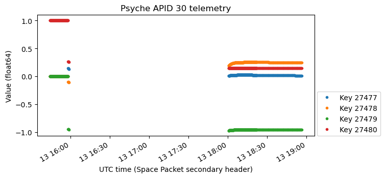
APID 107 transmits files that contain Space Packets from APID 30. The contents of these packets are the same as those of APID 10: telemetry in key-value format. It seems that APID 30 is the same data but recorded instead of real-time. It contains the same 4748 keys as APID 10.
As a quick comparison, the following plot shows the attitude quaternions from APID 30. The data after 18:00 UTC corresponds to the first file that was transmitted. The data before 16:00 UTC corresponds to the second file which was transmitted, which is incomplete because my observation with the ATA ended. Goldstone has a lower elevation mask than the ATA, so they would have continued tracking for more time, and then hand over seamlessly to Canberra. The rest of this file would probably complete all the missing telemetry until 18:00 UTC. The beginning of this file is 15:44:43 UTC. According to my notes, the spacecraft separation was 15:21 UTC.
For comparison, the quaternion telemetry from APID 10 received in real-time is shown again here.
APIDs 300, 318 and 1002
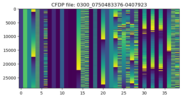
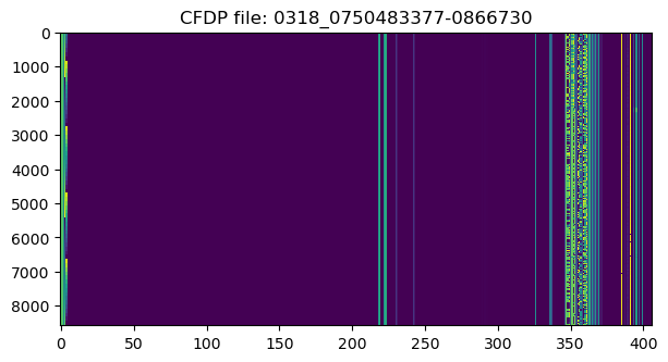
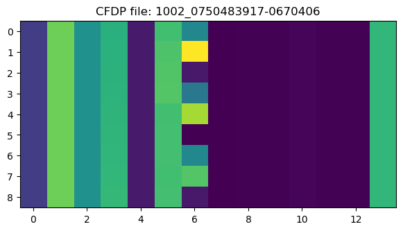
The files transmitted in APIDs 300, 318 and 1002 do not contain Space Packets. They contain segments of a fixed size which start by a spacecraft timestamp and then have some fixed format fields. The timestamp seems to be 40-bits long, with 1/256 second units elapsed since the J2000 epoch. In each file, the timestamps are regularly spaced.
Here are raster maps for one file in each of these APIDs. These show a quick overview of the field structure and contents.
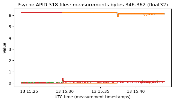
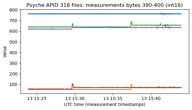
APID 318 is mostly filled with zeros, but there are some nonzero fields that are plotted below.
The contents of APID 1002 are too short to be able to make sense of the data.
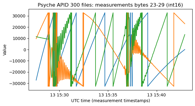
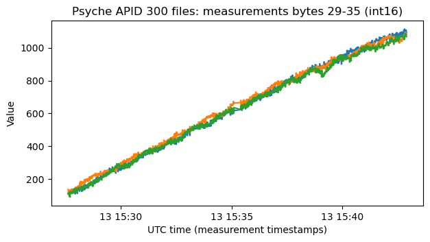
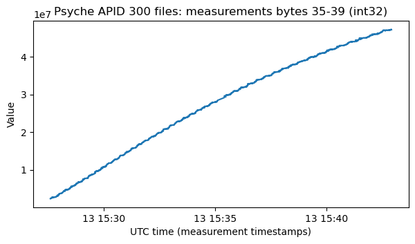
The following plots show the contents of some of the fields in APID 300. Note that the data starts shortly after spacecraft separation. I don’t know what any of these values represent. The values in the first plot are particularly interesting, because they wrap around, so they could be some kind of angle.
The next plot shows the values of some of the non-zero fields in the files in APID 318.
These are angles in radians, and it is perhaps better to wrap them to the range \([-\pi, \pi)\), since some of the values are close to zero and are constantly jumping between 0 and \(2\pi\) otherwise. I suspect that these values are related to the solar panel deployment, but the only reason I have for thinking this is that the times of the changes in the plot roughly matches the deployment, and that I imagine one solar array being deployed first, and then the other one.
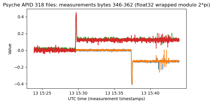
Some of the other fields contain related values, which show changes with the same shape.
Virtual channel 63
Virtual channel 63 is the only-idle-data virtual channel. It contains idle CCSDS Space Packets using M_PDU. The size of each packet fills up completely the M_PDU data zone, and each packet starts at the beginning of the data zone. The contents of each frame are identical except for the virtual channel frame count in the AOS frame and the packet sequence count in the Space Packets. The idle packets are constructed in the same way as in virtual channels 0 and 1, but these packets contain the full Easter egg message, while the packets in virtual channels 0 and 1 are cut short (they are only used to fill the remaining data zone in a partially filed frame). Idle packets for all the virtual channels seem to be drawn from the same source, in the sense that there is a global packet sequence count that increments regardless of the virtual channel in which the idle packet is transmitted.
As I advanced in the previous post, the payload of the idle packets is the following string, including line-feed characters. The length of the string is exactly the one needed to fill up completely the AOS frame with the idle packet. However observe that the length of the last line is shorter than the rest: one last space character and the line-feed are missing (you can see this by selecting the text to highlight the space characters).
A.Arslanian D.Beach M.Belete A.Bhosle Y.Brenman
D.Byrne R.Cheng P.Cheung M.Cisler D.Cummings
A.Dobrev P.Doronila B.Duckett D.Gaines L.Galdamez
L.Hall S.Harris H.Hartounian D.Hecox Q.Ho
J.Hofman Z.Hua C.Jones W.Kaye D.Kou S.Kroese
D.Leang L.Manglapus J.Masci B.Morin R.Nemiroff
C.Oda J.Pavek V.Reddy J.Sawoniewicz
A.Shearer L.Stewart G.Sun J.Thoma D.Tran R.Tsao
M.Tuszynski I.Uchenik M.Wade V.Wong R.Woo M.Yang
W.Yasin H.Yun ** Rohan the Destroyer b.12/9/21 **
        @@&J!~...       ^$$~      ^JPG@@@
        @#7!: .       ..~$$~     ^Y ~PP@@
        &77:..      :$$J: '     .5:  !##@
        Y!~.:      !J^ ~P ''    J5    G#&
        77:    !. !Y:   ~7!!7JY^^!Y   $&#
        77:    !.:5!         :^. ~~   $##
        5!~    ~:!5J777$$!            G#&
        @$7^    .^!JJJ$:5P.       ^^ $##@
        @&J$^      :.   YG.     .:J7J##@@
        @@@5$!.    :..  P&.   ^.!!!L.Park
           This spacecraft is equipped
    with the latest ABS and pDMA technologies
Code and data
The code and data used in this post is in this repository. It contains the binary files with the decoded AOS frames, as well as the Jupyter notebook where all the data analysis was done.
One comment