On Friday, the Psyche mission launched on a Falcon Heavy from Cape Canaveral. This mission will study the metal-rich asteroid of the same name, 16 Psyche. For more details about this mission you can refer to the talk that Lindy Elkins-Tanton, the mission principal investigator, gave a month ago at GRCon23.
The launch trajectory was such that the spacecraft could be observed from the Allen Telescope Array shortly after launch. The launch was at 14:19 UTC. Spacecraft separation was at 15:21 UTC. The spacecraft then rose above the ATA 16.8 degree elevation mask in the western sky at 15:53 UTC. However, the signal was so strong that it could be received even when the spacecraft was a couple degrees below the elevation mask, so I confirmed the presence of the signal and started recording a couple minutes earlier. At this moment, the spacecraft was at a distance of 18450 km. The spacecraft continued to rise in the sky, achieving a maximum elevation of 32.9 degrees at 16:53 UTC, and setting below the elevation mask on the west at 19:22 UTC. At this moment the spacecraft was 103800 km away. The signal could still be received for a few minutes afterwards, but eventually became very weak and I stopped recording.
Since the recording started only 30 minutes after spacecraft separation, we get to see some of the events that happen very early on in the mission. Most of the observations of deep space launches that I have done with the ATA have started several hours after launch. This Twitter thread by Lindy Elkins-Tanton gives some insight about the first steps following spacecraft separation, and I will be referring to it to explain what we see in the recording.
I intend to publish the recordings in Zenodo as usual, but the platform has been upgraded recently and is showing the following message “Oct 14 12:03 UTC: We are working to resolve issues reported by users.” So far I have been unable to upload large files, but I will keep retrying and update this post when I manage.
Update 2023-10-19: Zenodo have now solved their problems and I have been able to upload the recordings. They are published in the following datasets:
Recording and post processing
I recorded at 4.096 Msps 16-bit IQ centred on 8417 MHz. As I will explain below in more detail, at some point I lost the signal, and suspecting that my antenna pointing could be slightly off, I stopped the recording to search in real time for the signal. Doing this I realized that the signal loss was caused by the spacecraft attitude and not the groundstation antenna pointing. I began recording again as soon as I saw the signal again. Therefore, there are two recording files, with a gap between them in which the signal could not be received from Earth.
To point the antennas I used the ephemerides from HORIZONS, which contained a pre-launch trajectory. I prepared a custom antenna pointing file, as I did for OSIRIS-REx, using this data. In this case this was quite necessary, because the spacecraft was near enough that its right ascension and declination coordinates changed fast. When observing other deep space launches, maybe around 8 to 12 hours after launch, the right ascension and declination coordinates change slowly enough that I can update them every 10 minutes or so, either by hand or with a simple script.
I used antennas 1a and 5c from the ATA, which have the so called “old feeds”, and recorded the two linear polarizations from each antenna. Since I recorded for almost 4 hours, the total size of the recordings is too large to publish in Zenodo.
During most of the time the spacecraft was transmitting a low rate 12 kbaud signal. I have decimated the recordings to 128 ksps centred on 8417.525 MHz. This is more than enough to process this telemetry signal and reduces the file size significantly, so I can publish the four channels (2 antennas and 2 polarizations) in a Zenodo dataset.
For the last 90 minutes of the recording, there are some signals of interest in a larger bandwidth. First, sequential ranging begins with tones approximately 1 MHz away from the carrier. Then the modulation changes to a much faster 366.66 kbaud. What I have done is to convert this part of the recording to 8-bit IQ without decimation, and I will publish only one antenna and polarization in Zenodo. The signal is strong enough that it is sufficient to use a single linear polarization.
Waterfall analysis
I have reused most of waterfall plotting code that I did for OSIRIS-REx a couple weeks ago. The following figure shows the waterfall of the two recordings.
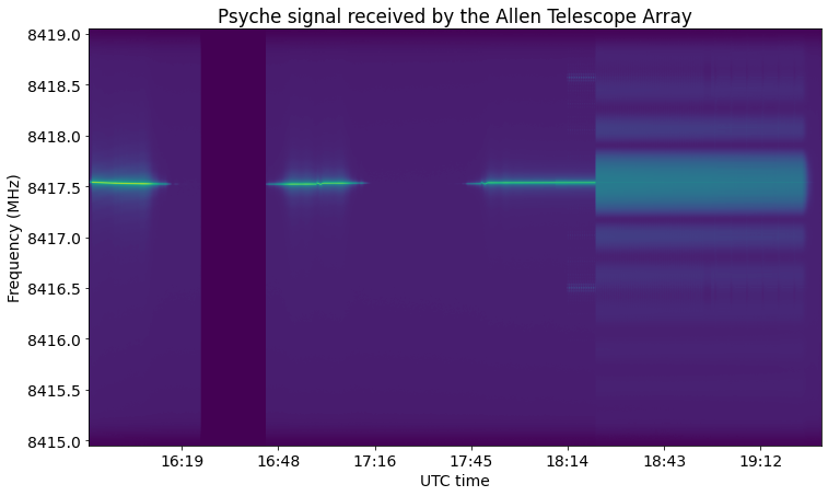
The dark purple gap around 16:30 corresponds to when I stopped recording to try to search for the signal. In the waterfall we can clearly see that the spacecraft signal fades out smoothly around 16:30 and 17:30. This is caused by the spacecraft “rotisserie” mode, which if I understood correctly Lindy’s Twitter thread, consists in the spacecraft pointing its +X axis towards the Sun and spinning slowly around it. The solar panels are located along the Y axis and can rotate about this axis, so in this situation they can be pointed directly towards the Sun. Presumably, in this situation the spacecraft would be using the -Z low-gain antenna (there are low gain antennas on the +X, -X and -Z faces, and then high gain antenna on in the +Z face, with the boresight pointing at an offset of 10 deg with respect to the +Z axis). Thus, the -Z LGA will periodically come in an out of view from Earth as the spacecraft rotates slowly. In the next post I will look at this in more detail, since I have already found the spacecraft attitude quaternions and other ADCS data in the telemetry, and can relate them to what appears in the waterfall.
In any case, when I was recording I didn’t have all the information about the rotisserie mode, and suspected that I might have lost the signal because the antenna pointing was wrong. At X-band, the ATA antennas have a beamdwidth of 0.2 deg, and sometimes the pre-launch trajectory data is not accurate enough to track without some manual tweaking of the antenna pointing by a fraction of a degree. In this case the pre-launch trajectory on HORIZONS turned out to work pretty well for antenna pointing, and after seeing the signal reappear and confirming that the pointing was good, I realized that the loss of signal was due to the spacecraft attitude, and that I could consider the antenna pointing to be good. When the signal was lost again, I simply continued recording waiting for it to appear again. There are no more signal drops because, as we will see in the telemetry, the spacecraft stopped the rotisserie mode at around 18:00 UTC.
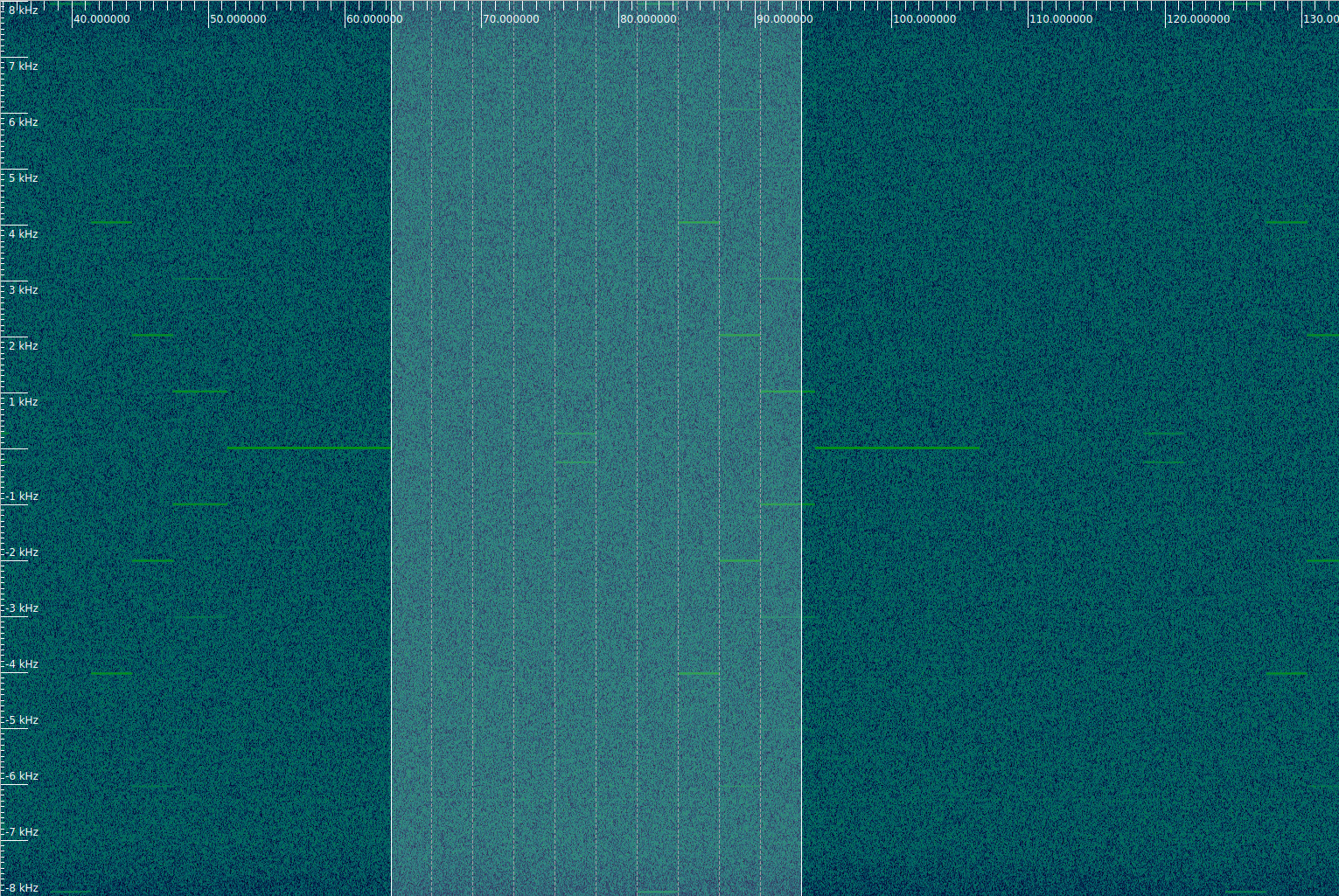
Besides the periodic fading of the signal, there are other events that we can see in this waterfall. At around 18:15 UTC, sequential ranging tones appear at an offset of approximately 1 MHz from the signal. The modulation changes to a much higher rate shortly after. We also see the uplink sweeps corresponding to two groundstation locks. These are best seen in the figure blow, which shows a zoom to the frequency range around the low rate signal. One of the groundstation locks happens around 17:00 UTC, in the middle of one of the periods of visibility of the spacecraft signal. The other lock happens around 17:50, shortly after the signal becomes visible again.
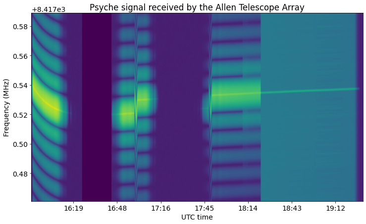
Another thing that we can see in this figure is that the spacecraft transponder turns on at around 18:00. The transponder noise can be seen to appear suddenly. Some minutes later sequential ranging begins.
Modulation and coding
The modulation for both the low rate signal and the high rate signal is PCM/PM/NRZ. This means that the telemetry baseband is directly modulated using phase modulation with residual carrier. The symbol rate is 12 kbaud for the low rate signal and 366.66 kbaud for the high rate signal. It is somewhat uncommon to use baseband modulation (instead of subcarrier modulation) for a symbol rate as low as 12 kbaud. The reason to avoid this is that at low symbol rates the telemetry modulation interferes with the PLL that locks to the residual carrier, unless the PLL bandwidth is narrow. I have observed that a PLL bandwidth of 100 Hz produces significant interference on the PLL, so I have used a bandwidth of 10 Hz with the low rate signal.
The coding is always r=1/6 CCSDS Turbo code with 1115 byte frames. This choice of coding gives the best Eb/N0 performance among those listed by the CCSDS TM Synchronization and Channel Coding Blue Book.
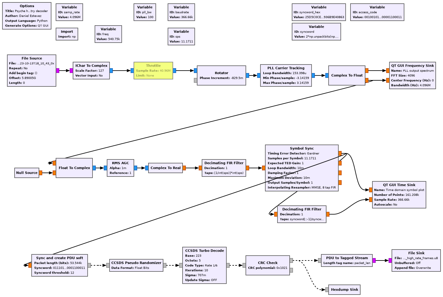
The following figure shows a GNU Radio flowgraph to decode the low rate signal. It uses some blocks from gr-satellites and the Turbo decoder from gr-dslwp.
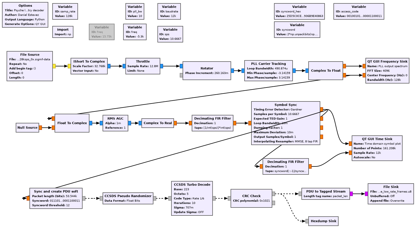
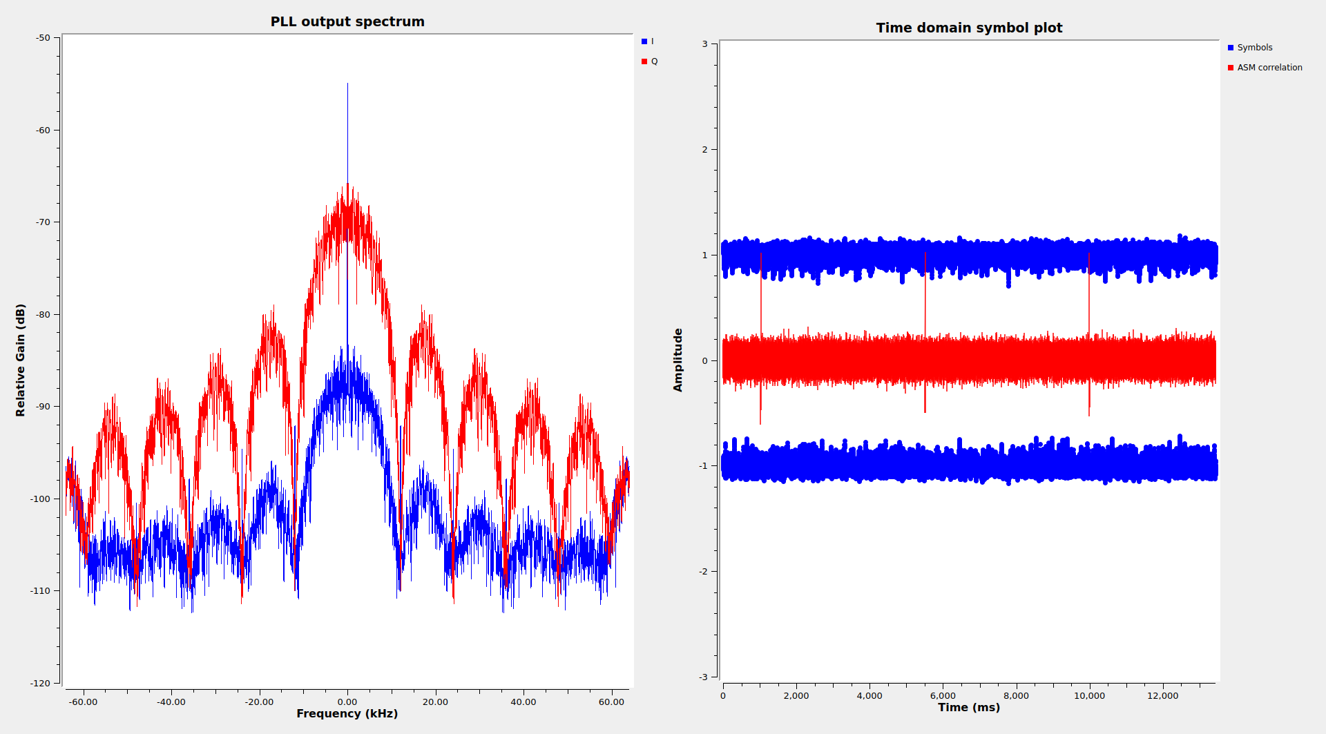
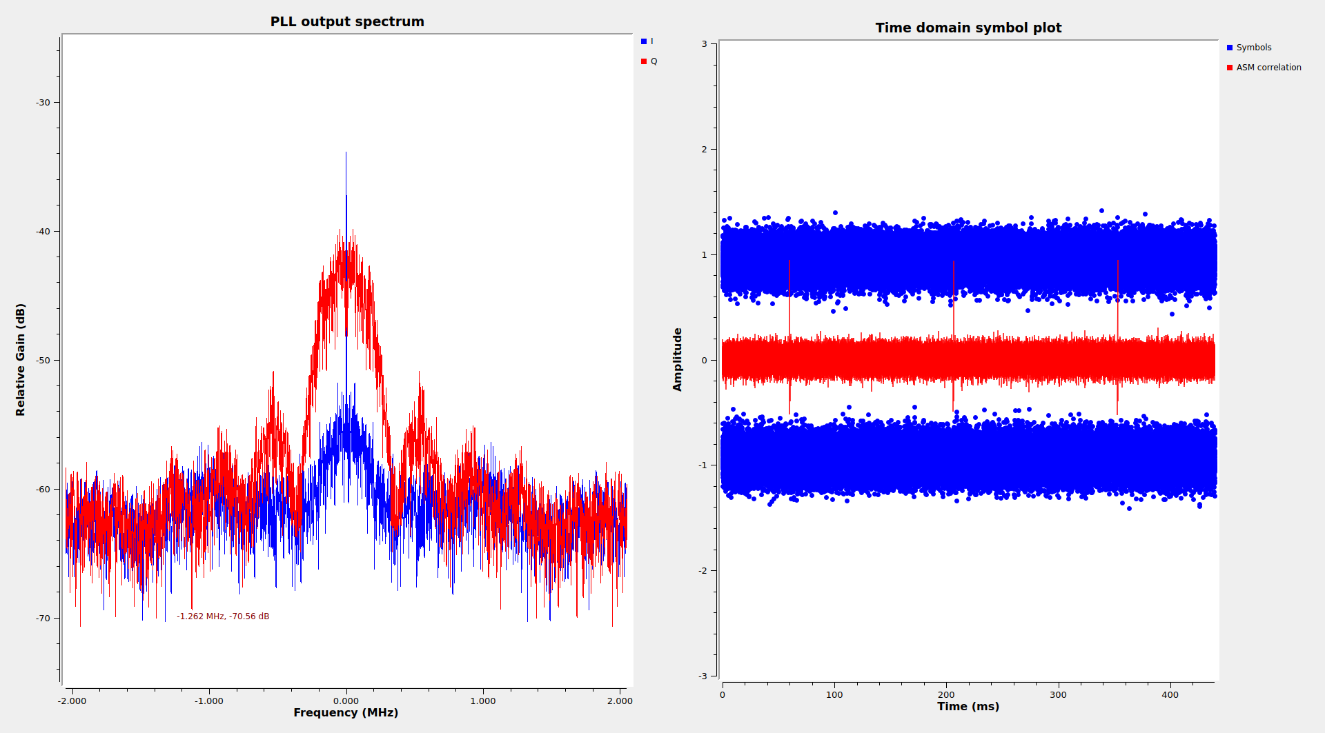
Here is the GUI of the flowgraph running on the recording. The SNR is excellent. There is some leakage of the telemetry modulation in the in-phase component of the PLL output. This is caused because the presence of a significant amount of modulation power in the PLL loop bandwidth introduces jitter in the PLL. Increasing the PLL bandwidth makes things even worse.
The GNU Radio decoder for the high rate signal is very similar. The only difference is the symbol rate (and the input sample rate, since I am using it with the 4.096 Msps recording), and the PLL bandwidth, which I have set to 100 Hz in this case.
Uplink sweep
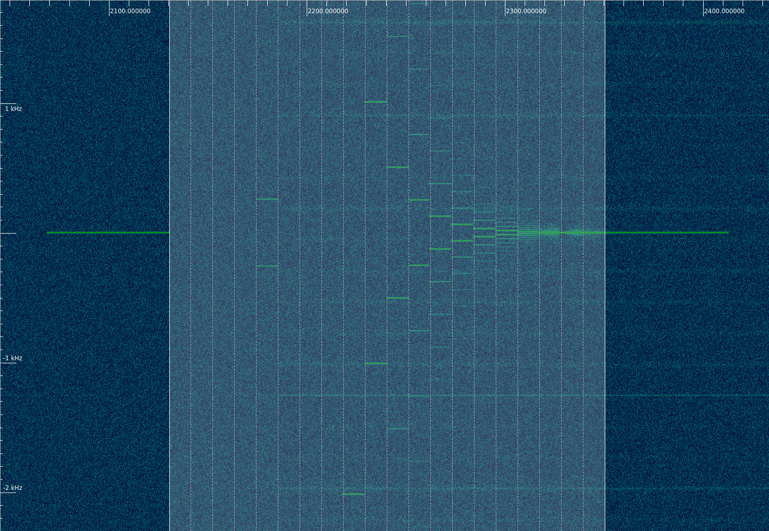
We have seen in the waterfall that there are two uplink sweeps in the low rate signal. These are best viewed in Inspectrum, which displays the waterfall shown here.
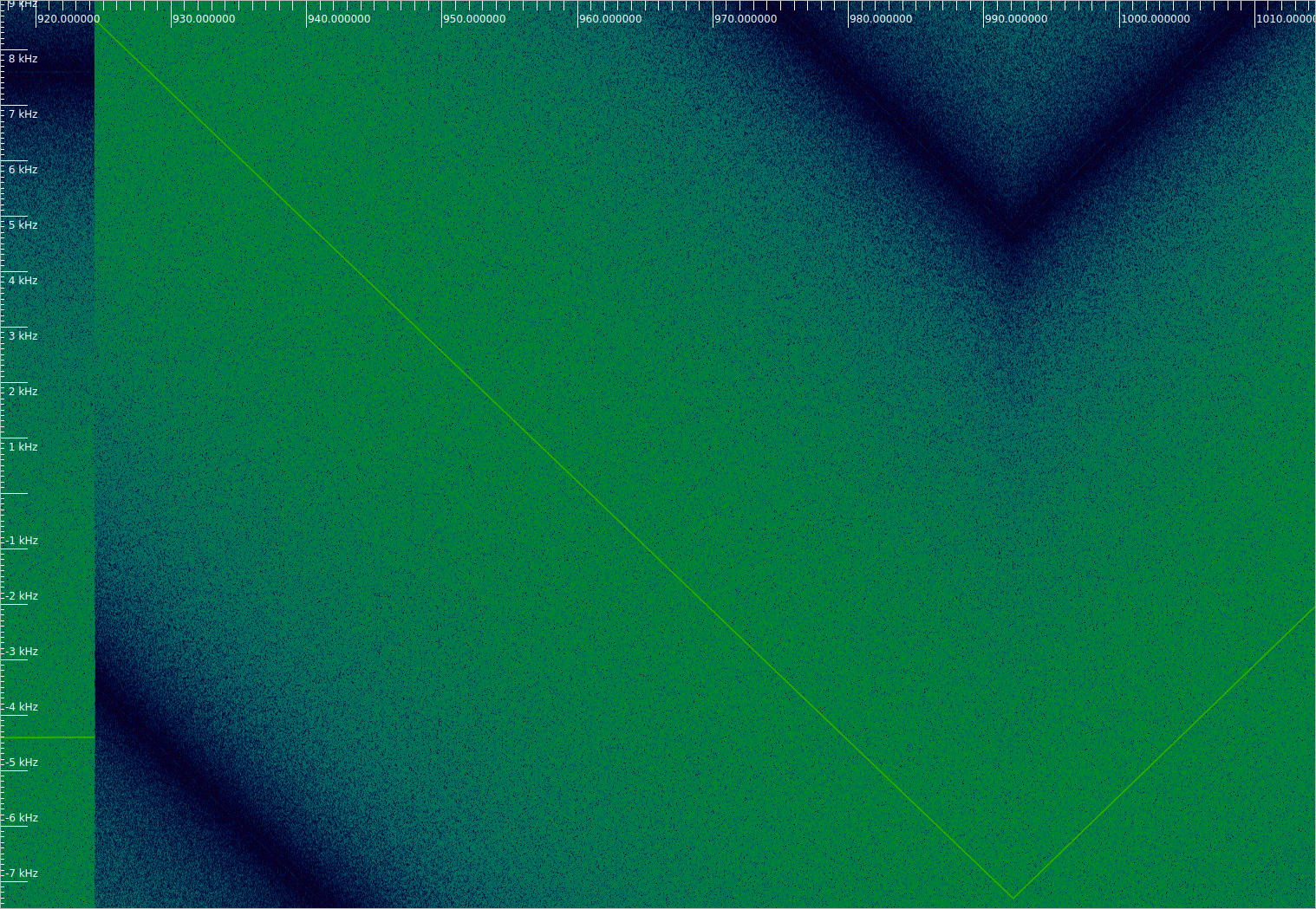
The pattern in both sweeps is the same. First the spacecraft signal jumps up by 11.8 kHz. This happens because the uplink is sweeping down and the spacecraft receiver PLL first locks when the frequency error is below 11.8 kHz (or actually, 11.8 kHz divided by the transponder turnaround frequency ratio). Then the sweep goes down at a rate of approximately 236 Hz/s for 68 seconds, decreasing 16 kHz in frequency. Finally, it sweeps up at a rate of 236 Hz/s for 50 seconds, increasing in frequency by 11.8 kHz.
Sequential ranging
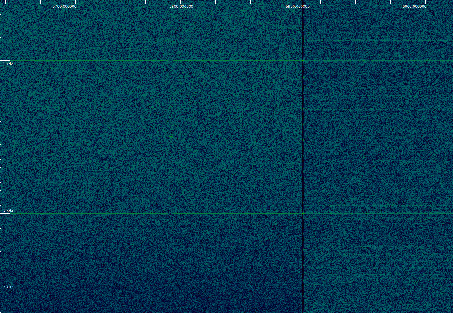
A closer look to the sequential ranging tones reveals that there are actually two different sequential ranging measurement configurations being used. The first one is used until 18:43 UTC, and the second one starts at 18:45 UTC and continues until 19:12 UTC.
Both configurations use a ranging clock of approximately 1032.201 kHz (the exact value depends on the uplink frequency and Doppler). This is component number 4, which corresponds to a frequency of \(2^{-11}f_U/749\), where \(f_{U}\) is the X-band uplink frequency (see the DSN Telecommunications Link Design Handbook chapter on sequential ranging for the relevant formulas and terms).
In the first ranging configuration, the ranging clock is transmitted for 12 seconds, the remaining tones except the last are transmitted for 3 seconds, and the last tone, which is the ranging clock divided by \(2^{10}\) (component 14), is transmitted for 4 seconds. Starting with the ranging clock divided by \(2^2\), the tones use chopping. A complete measurement with this configuration takes 43 seconds.
In the second ranging configuration, the ranging clock is transmitted for 63 seconds, and the remaining tones are transmitted for approximately 11 seconds, although there appears to be some small variation. The last tone is equal to the ranging clock divided by \(2^{20}\) (component number 24). As in the first configuration, starting with the ranging clock divided by \(2^2\) the tones are chopped. A complete measurement takes 282 seconds. Only 6 full measurements plus the ranging tone of the next one are done in this configuration.
Since the first configuration goes until component 14, according to Table 1 in the DSN handbook it has an ambiguity resolution of 148 km. The second configuration goes until component 24, so it has an ambiguity resolution of 152221 km. I am curious for the motivation to use these two different ranging configurations. The first configuration seems sufficient for orbit determination in this mission phase. Given that the second configuration goes until the last component that can ever be used (which is not justified by the range uncertainty that there is at this moment), and that it uses significantly longer tone durations than the first one, it is perhaps intended as an accurate characterization of the spacecraft transponder performance for sequential ranging purposes.
Telecommand subcarrier
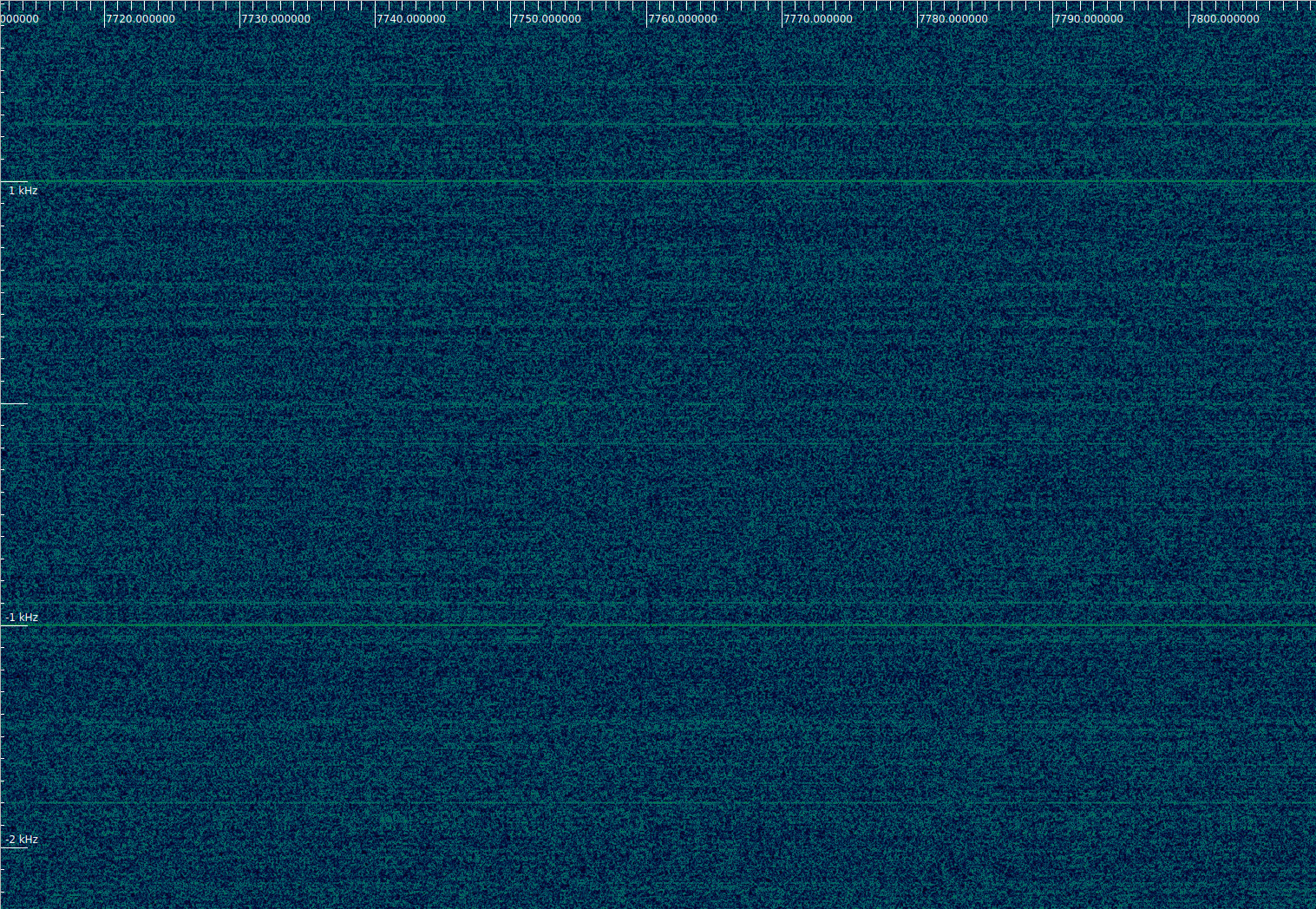
Starting at 18:10:46 UTC the telecommand subcarrier is visible in the spacecraft transponder. This seems to be the moment when the transponder turns on, so the telecommand might have been modulated on the uplink already before this. The telecommand subcarrier is 16 kHz, and the symbol rate is 2 kbaud.
Most of the time the telecommand subcarrier is idle. At 18:20:48 UTC, a telecommand is sent. This happens a couple minutes before the telemetry modulation change. Both can be seen in the figure below. It stands out that the telecommand packet has some residual carrier. Since it is BPSK-modulated, this would happen if the data is unbalanced (there are more zeros than ones or vice versa).
I have seen another telecommand sent at 18:53:20 UTC. This one is more difficult to see because it is shorter and happens during the high rate modulation, which seem to to rob some downlink power from the transponder.
Telemetry
A detailed analysis of the telemetry will be done in a future post, since it will take me more work to complete it. The telemetry frames of Psyche are AOS frames containing Space Packets, and in some ways the telemetry is similar to that of OSIRIS-REx (more or less the same APIDs are used, and the data has a key-value structure, though maybe I’m just realizing this similarities because OSIRIS-REx is the latest NASA spacecraft I analyzed). A remarkable thing about the telemetry is that the idle packets, which are also used to fill up virtual channel 63 (the only-idle-data virtual channel) contain the following easter egg in ASCII. If you are curious about who are these people, many of the names appear in the list of the Psyche team.
A.Arslanian D.Beach M.Belete A.Bhosle Y.Brenman
D.Byrne R.Cheng P.Cheung M.Cisler D.Cummings
A.Dobrev P.Doronila B.Duckett D.Gaines L.Galdamez
L.Hall S.Harris H.Hartounian D.Hecox Q.Ho
J.Hofman Z.Hua C.Jones W.Kaye D.Kou S.Kroese
D.Leang L.Manglapus J.Masci B.Morin R.Nemiroff
C.Oda J.Pavek V.Reddy J.Sawoniewicz
A.Shearer L.Stewart G.Sun J.Thoma D.Tran R.Tsao
M.Tuszynski I.Uchenik M.Wade V.Wong R.Woo M.Yang
W.Yasin H.Yun ** Rohan the Destroyer b.12/9/21 **
        @@&J!~...       ^$$~      ^JPG@@@
        @#7!: .       ..~$$~     ^Y ~PP@@
        &77:..      :$$J: '     .5:  !##@
        Y!~.:      !J^ ~P ''    J5    G#&
        77:    !. !Y:   ~7!!7JY^^!Y   $&#
        77:    !.:5!         :^. ~~   $##
        5!~    ~:!5J777$$!            G#&
        @$7^    .^!JJJ$:5P.       ^^ $##@
        @&J$^      :.   YG.     .:J7J##@@
        @@@5$!.    :..  P&.   ^.!!!L.Park
           This spacecraft is equipped
    with the latest ABS and pDMA technologies
Code and data
The Jupyter notebook used to plot the recording waterfalls and the GNU Radio flowgraphs used for data reduction can be found in this repository. The GNU Radio decoder flowgraphs are in this repository. The recordings in Zenodo are listed at the beginning of the post.
2 comments