On September 24, the OSIRIX-REx sample return capsule landed in the Utah Test and Training Range at 14:52 UTC. The capsule had been released on a reentry trajectory by the spacecraft a few hours earlier, at 10:42 UTC. The spacecraft then performed an evasion manoeuvre at 11:02 and passed by Earth on a hyperbolic orbit with a perigee altitude of 773 km. The spacecraft has now continued to a second mission to study asteroid Apophis, and has been renamed as OSIRIS-APEX.
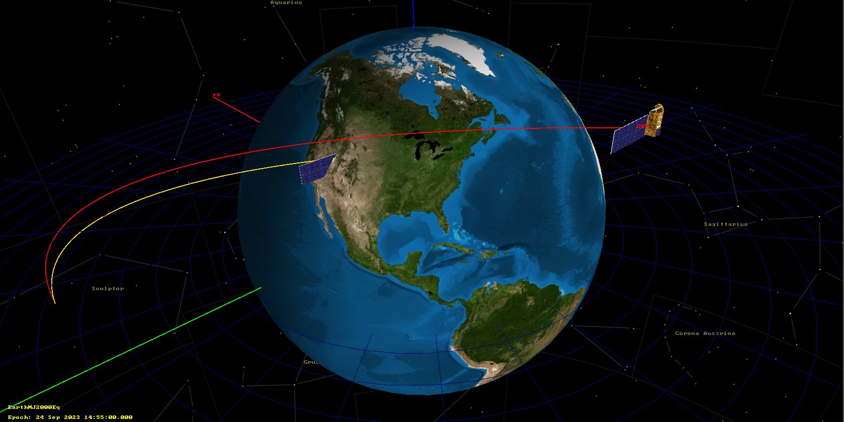
This simulation I did in GMAT shows the trajectories of the spacecraft (red) and sample return capsule (yellow).
Since the Allen Telescope Array (ATA) is in northern California, its location provided a great opportunity to observe this event. Looking at the trajectories in NASA HORIZONS, I saw that the sample return capsule would pass south of the ATA. It would be above the horizon between 14:34 and 14:43 UTC, but it would be very low in the sky, only reaching a peak elevation of 17 degrees. Apparently the capsule had some kind of UHF locator beacon, but I had no information of whether this would be on during the descent (during the sample return livestream I then learned that the main method of tracking the capsule descent was optically, from airplanes and helicopters). Furthermore, the ATA antennas can only point as low as 16.8 degrees, so it wasn’t really possible to track the capsule. Therefore, I decided to observe the spacecraft X-band beacon instead. The spacecraft would also pass south of the ATA, but would be much higher in the sky, reaching an elevation above 80 degrees. The closest approach would be only 1000 km, which is pretty close for a deep space satellite flyby.
As I will explain below in more detail, I prepared a custom tracking file for the ATA using the SPICE kernels from NAIF and recorded the full X-band deep space band at 61.44 Msps using two antennas. The signal from OSIRIS-REx was extremely strong, so this recording can serve for detailed modulation analysis. To reduce the file size to something manageable, I have decimated the recording to 2.048 Msps centred around 8445.8 MHz, where the X-band downlink of OSIRIS-REx is located, and published these files in the Zenodo dataset “Recording of OSIRIS-REx with the Allen Telescope Array during SRC reentry“.
In the rest of this post, I describe the observation setup, analyse the recording and spacecraft telemetry, and describe some possible further work.
Observation setup
Since this was an observation of a low altitude Earth flyby, it is quite different from the usual observations of deep space satellites that I do with the ATA. It is much more similar to a pass of a LEO satellite. In deep space observations the satellite is visible for several hours, giving a lot of time to confirm the signal SNR, frequency and bandwidth before recording. Also, the right ascension and declination coordinates change slowly, which makes tracking quite easy (I often copy right ascension and declination coordinates from HORIZONS every 15 minutes or so, or even a single time for the whole observation).
In this case, the OSIRIS-REx pass lasts only around 7 minutes, so it is not possible to check things manually and correct the antenna pointing if something is wrong. The trajectory for the antenna tracking needs to be prepared beforehand and the recording is started and stopped at the expected times of acquisition of signal and loss of signal. Only after the pass ends we can look at the recording and find out if it was good. An event like this gives a single opportunity for observing, so it is good to prepare the observation carefully and do some tests to ensure that everything will work correctly.
In the case of this observation, I used a custom antenna tracking file for the ATA. This file lists the antenna azimuth and elevation as a time series (using TAI in nanoseconds as the time variable). To prepare the file, I used SPICE kernels with SpiceyPy in this Jupyter notebook. I obtained the SPICE kernels from the NAIF repository for ORX. The SPK (spacecraft trajectory kernel) that I used was orx_230117_231101_230911_od368-N-TCM12-P-DB1_v1.bsp, which was the latest one available on 2023-09-24. The description for this kernel can be read here. The kernel was prepared on 2023-09-11 using preliminary planning for the TCM12 manoeuvre, which would happen on 2023-09-17.
I was a bit nervous about not having more up to date trajectory data for this observation (in particular data including orbit determination after TCM12), because since the pass closest approach would be only 1000 km, an error of just 3.5 km in the trajectory would cause an angular error of 0.2 deg, which is the beamwidth of the ATA dishes at 8.45 GHz. Nevertheless, the observation turned out quite well using this trajectory data, and it appears that the spacecraft was inside the dishes primary beam. Since I am interested in measuring the trajectory more accurately, I recorded using two antennas with a relatively long baseline (around 250 meters), and also observed the quasar 3C84 before and after the OSIRIS-REx pass, to use it as a calibrator. I haven’t done any interferometric analysis in this post, so this will probably be the topic for a future post.
To use SPICE to calculate the spacecraft azimuth and elevation as seen from the ATA, I needed to make SPK and FK kernels for a topocentric frame for the ATA. For this, I used the pinpoint utility and the following definitions:
\begindata

   SITES = ( 'ATA' )
   ATA_FRAME = 'ITRF93'
   ATA_CENTER = 399
   ATA_IDCODE = 399999
   ATA_LATLON = ( 40.8175, -121.4733, 1.008 )
   ATA_UP = 'Z'
   ATA_NORTH = 'X'

\begintext
Since the object code that I used for the ATA is not standard, I also needed to define it in SpiceyPy using sp.boddef('ATA', 399999).
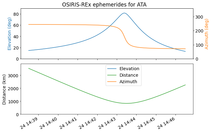
The plot below shows the azimuth, elevation and distance of OSIRIS-REx computed with SPICE. With this data I made the custom antenna ephemeris file for the ATA.
The ATA antennas are fast enough to track most LEO passes, but a 700 km altitude hyperbolic orbit pass near periapsis is faster, so I wanted to test the antennas to see if they could keep up with the ephemeris file. For this, I run some tests on the day before the sample capsule return. Basically, I translated in time the ephemeris file and made the antennas track as if it was the real pass, measuring their azimuth and elevation in real time and then comparing to the ephemeris file.
I found that the antennas could track correctly during most of the pass, but they weren’t fast enough in azimuth during the 30 seconds of maximum elevation. The plot below shows the azimuth of the antennas during one of the tests compared to the ephemeris file. I measured the pointing of the antennas by polling the ATA REST API every 100 ms. However, it seems that the value returned by this API does not refresh quickly enough, which causes a visible staircase pattern. In any case, it is clear that during the maximum elevation part of the pass the antennas are lagging by many degrees.
On the other hand, tracking in elevation seemed accurate, taking into account that we should only look at the points when the staircase pattern changes, since the rest of the time the same value is held constant by the REST API.
Recording waterfall
As I have mentioned, I recorded at 61.44 Msps centred at 8425 to cover all the 8.40 – 8.45 GHz deep space X-band allocation. Although I knew that the OSIRIS-REx frequency was around 8446 MHz, since I didn’t have a way of confirming this during the observation, I decided to record all the 50 MHz wide deep space allocation, just in case there were unexpected signals. To check the quality of the recording I computed waterfall data using a GNU Radio flowgraph and plotted the waterfall and spectrum using a Jupyter notebook.
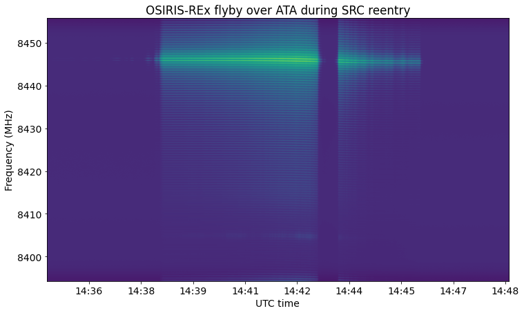
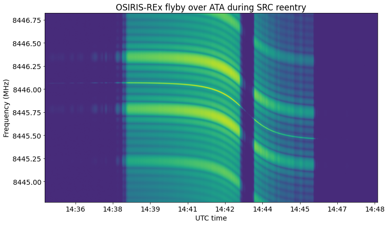
The following figure shows the waterfall of antenna 1a polarization X. I started the recording a few minutes before the expected acquisition of signal, and finished a few minutes after the expected loss of signal. During the beginning and end of the recording the antennas were pointing to the location where the spacecraft would cross the 16.8 degree elevation mask (this is what the ATA system does automatically). We can see that the signal appears more or less when expected, becomes very strong, is lost when the antennas cannot keep up, then is received again, and finally gets lost.
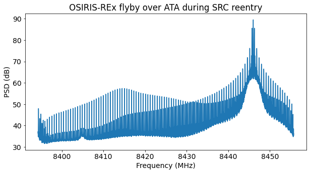
The next figure is the spectrum of the signal at the midpoint of the recording. The SNR is extremely high.
If we zoom in frequency in the waterfall we can see the Doppler on the carrier and sidebands.
A zoom to the spectrum is quite interesting. We see sidebands at odd harmonics of the subcarrier frequency, which is typical for a square wave subcarrier. However, at some point we also see even harmonics start to appear. These are unmodulated because the BPSK modulation of the telemetry subcarrier disappears on even harmonics. The reason why these even harmonics are present is because the telemetry signal (including the subcarrier) is not a perfect square wave. It takes some small amount of time to slew between its positive and negative values. Since the telemetry signal phase-modulates the carrier, this slew mainly causes an amplitude modulation of the residual carrier at a frequency of twice the subcarrier frequency. This manifests as tones at multiples of twice the subcarrier frequency which are in phase with the residual carrier.
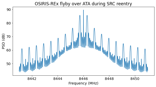
This reasoning explains better what we see in the plot over the full bandwidth. The odd harmonics of the telemetry subcarrier drop off at the expected 1/f rate for a square wave. However, the even harmonics start to increase in power at some point and follow an interesting curve, becoming stronger than the odd harmonics. The relation of the powers of all these harmonics tells us the details of the pulse shape of the telemetry. This recording is ideal for this kind of modulation analysis because it has a wide bandwidth and very high SNR.
Another thing that is visible in the spectrum is a wideband noise hump approximately 4 MHz wide and centred on the residual carrier. I think that this is the spacecraft transponder, which is simply retransmitting thermal noise at its receiver input.
It is important to keep in mind that during this observation there was no uplink signal. To my knowledge, only the ATA was tracking OSIRIS-REx. The DSN antennas are not fast enough to track this kind of pass. Therefore, this ATA observation gives a unique insight of the Earth flyby. Although this dataset does not have a huge scientific or engineering value for the mission, it can still be of interest.
Modulation and coding
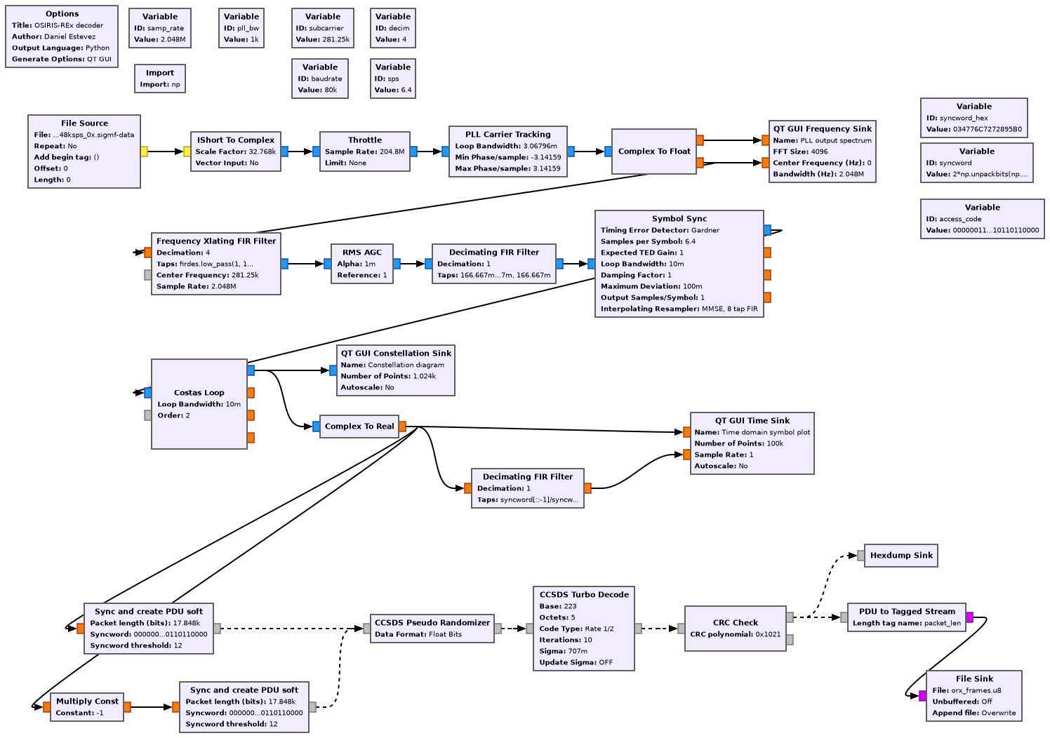
The modulation is PCM/PSK/PM (residual-carrier phase modulation with the subcarrier BPSK modulated on a subcarrier) with a subcarrier frequency of approximately 281.21 kHz and a symbol rate of 80 kbaud. Interestingly, the subcarrier frequency is close to 3.5 times the symbol rate, but not quite (usually the subcarrier is chosen to be an integer multiple of the symbol rate so that there is no telemetry modulation power at the residual carrier frequency). The coding is CCSDS Turbo code with rate 1/2 and 1115 information bytes frames.
The following figure shows the GNU Radio flowgraph that I have used to decode the telemetry signal. Since the SNR is very good, I am only using one polarization and antenna. A relatively large PLL bandwidth of 1 kHz is used to be able to track the large Doppler drift near the centre of the pass. This flowgraph uses some blocks from gr-satellites and gr-dslwp.
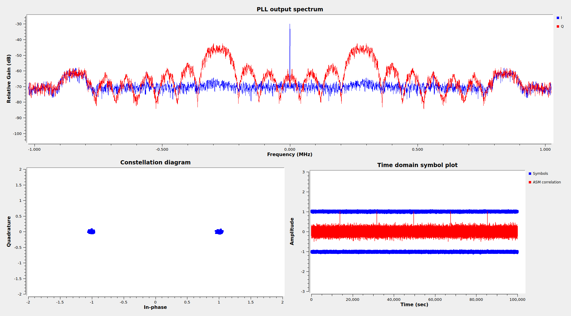
The GUI of the flowgraph shows that the SNR is extremely good during most of the pass. The constellation diagram has very little noise.
AOS frames
OSIRIS-REx uses CCSDS AOS Transfer Frames with a Frame Error Control Field (CRC-16). The Frame Error Control Field is checked by the GNU Radio decoder flowgraph. The spacecraft ID is 0x40, which matches the SANA registry. Virtual channels 0 and 63 (which is the Only Idle Data virtual channel) are in use in this recording. As usual, I have analysed the telemetry frames in a Jupyter notebook.
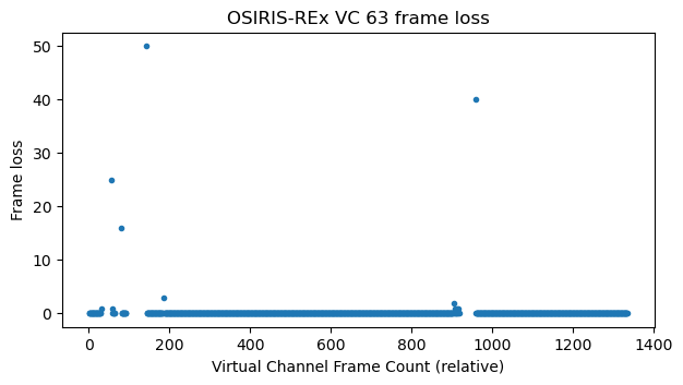
The following plots show the number of frames lost in each virtual channel, computed by using the virtual channel frame count field. There are some frames lost at the beginning, when the signal starts to appear, and also when the antennas could not keep up.

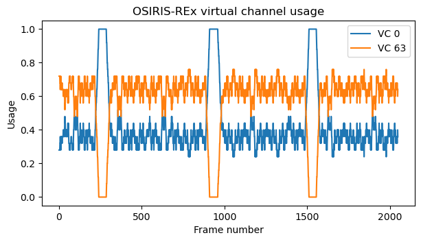
The usage share for the virtual channels is shown here. We see that virtual channel 0, which transmits the useful data, only takes up about 30% of the utilization most of the time. There are three events where the utilization for virtual channel 0 spikes up to 100%. We will see below what these are.
The frames in virtual channel 63 contain a first header pointer value of 0x7fe in the M_PDU header. This indicates only idle data. The packet zone is filled with 0xaa bytes.
There is no secondary header or Operational Control Field in the AOS frames.
Virtual channel 0
Real-time telemetry is transmitted in Virtual Channel 0 using CCSDS Space Packets in M_PDU. All the packets have a 5 byte secondary header which contains a timestamp. The timestamp is given as a 5 byte big-endian integer that nominally counts the number of 1/256 second units elapsed since the J2000 epoch. As we can imagine, the spacecraft on-board clock has some error, and information about this is given by the SCLK SPICE kernels. The latest kernel contains the following measurement of the spacecraft clock:
# *____SCLK0_______  ____SCET0____________ _DUT__ _SCLKRATE___
# 0744187124.000    2023-213T18:40:28.544 69.184 01.000000492
This means that the spacecraft clock 0744187124.000 (seconds since the J2000 epoch) actually corresponds to (spacecraft even time) 2023-08-01T18:40:28.544 UTC. Therefore, the on-board clock is wrong by 104.544 seconds. When converting the Space Packet timestamps to UTC time I have ignored the spacecraft clock rate, though that would have accumulated to approximately 2 seconds by the end of September. If the precise UTC timestamp of each frame was needed, SpiceyPy could be used with this kernel to convert spacecraft clock values to UTC.
In this recording, APIDs 3, 4, 5, 6, and 2047 (the idle APID) are used. Idle packets in APID 2047 are filled with 0x55 bytes. The remaining APIDs have packets of variable length and carry telemetry values using a key-value format. The payload of each packet is a concatenation of pairs of a 16-bit key followed by a value, which can be either 8, 16, 32 or 64 bits long. The length of the value seems to be conveyed implicitly by the key, since I didn’t found any pattern in the keys that would correlate to their corresponding field lengths.
A decoder for this kind of key-value format knows the set of all the keys and their corresponding value lengths, so it can parse all the data. When reverse engineering, it is usually not too difficult to parse this format by hand. The numbers of the keys that tend to appear are in an increasing order, often without large jumps, and are related to their function. For instance, if some telemetry value is a vector with 3 components, these will appear in three keys with consecutive numbers that are transmitted sequentially. So one can simply look at the binary data and decide what part of the data is the keys, and so what are the lengths of each value.
I set out to do this kind of work by hand with the OSIRIS-REx telemetry before realizing that there is actually a huge number of different keys being used (14052, to be precise). This means that even though relatively straightforward, the process of making a table by hand of all the keys and their corresponding value lengths is very time consuming and tedious. There are some patterns in the way that keys and lengths appear that can save some work, though not that much. I regretted my decision of reverse engineering this key-value format when I realized the large amount of time it was taking me. Nevertheless, I decided to push on and finish (this is how I’m able to tell that there are exactly 14052 different keys). The table of keys and lengths I have made perhaps has a few small errors: it is possible to mistake two length 1 fields by a single length 4 field (both have a total length of 6 bytes), or a length 4 field and a length 2 field by a single length 8 field (both have a total length of 10 bytes). The table also contains some keys that are not actually present in the data (the table has 14703 keys), because sometimes I was a bit sloppy in avoiding to add missing keys. Having extra keys is not a problem for parsing the data, but reduces the chances of detecting mistakes when the length of a key has been set incorrectly.
I am not sure if making this table of keys of lengths by hand has been worth the effort. The time spent on this is the main reason why it has taken me two weeks to prepare this post. Perhaps it is possible to come up with some heuristics or machine learning algorithms that can do the same job correctly.
The maximum length of the Space Packets transmitted by OSIRIS-REx is 2048 bytes. When there is more data to be sent for this key-value structure, the data continues in the next Space Packet in the same APID. A single key-value pair is never split between two space packets. This explains why the packet size is quite irregular.
Another thing of interest is that there seems to be a glitch (or unusual mechanism) in the way in which Space Packets are fragmented into AOS frames using M_PDU. I noticed this because my Python reassembly code prints a warning (besides the warnings printed because of lost AOS frames). Upon closer look, the glitch seems to happen as follows. The last Space Packet in the frame with virtual channel frame count 1644628 in virtual channel 0 is an APID 2047 idle packet. There are only 6 bytes remaining in this frame, and the minimum size of a Space Packet is 7 bytes. This particular idle packet should have a length of 11 bytes (the length field value equals 4). Therefore, it should continue in the next frame of virtual channel 0. After this frame, an idle frame from virtual channel 63 is transmitted. Next we have virtual channel frame count 1644629 from virtual channel 0. However, the first header pointer of this frame is zero, and a new Space Packet starts right at the beginning of the packet zone. The remaining part of the idle space packet is missing.
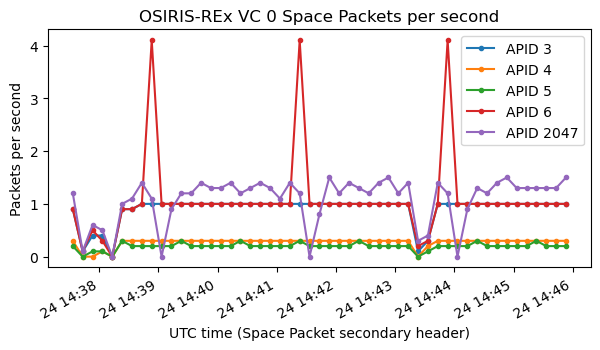
The following plot shows the number of packets per second transmitted on each APID, measured on 10 second averages. The drops around 14:38:00 and 14:35:30 are simply caused by lost AOS frames. We see that APIDs usually have a fixed reporting interval, such as one packet per second for APIDs 3 and 6, but on top of that APIDs 5 and 6 periodically send additional packets. In fact the 4 packets per second peaks of APID 6 correspond with the 100% utilization peaks of virtual channel 0 that we saw above.
The previous plot does not tell the whole story, because it doesn’t take into account the size of the packets. The following shows the bytes per second transmitted in each APID (counting Space Packet headers also). The vertical scale is logarithmic. The peaks on APID 6 correspond to large amounts of data (6.6 KB/s). We also see that the amount of idle data (around 1 KB/s) is fairly large, which makes sense, because many of these Space Packets are relatively short and there is no more useful data to fill the AOS frame.
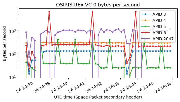
Additionally, we see that the data rate of APIDs 5 and 6 drops a little after 14:41:30. Since the number of packets per second seems unaffected, this means that shorter packets start to be sent. This seems to be caused by some configuration or operational change on the telemetry that gets reported. I don’t know what causes this change, but we will see more about it when we look at the data in each APID.
APID 3
APID 3 is the easiest one to parse. In fact, it is not necessary to parse it using the key-value structure, because the fields in the packets always line up, as it can be seen in the raster map below. The only variability in the format of these packets is whether the last key-value (key 33880) is present or not. This last field seems to be present only every 8 packets. It can be seen in the raster map. The shorter packets have been padded with zeros to the size of the longest packet. These zeros are shown in dark purple in the raster map. Thus, the packets with the extra field are those that end with some green-blue data.
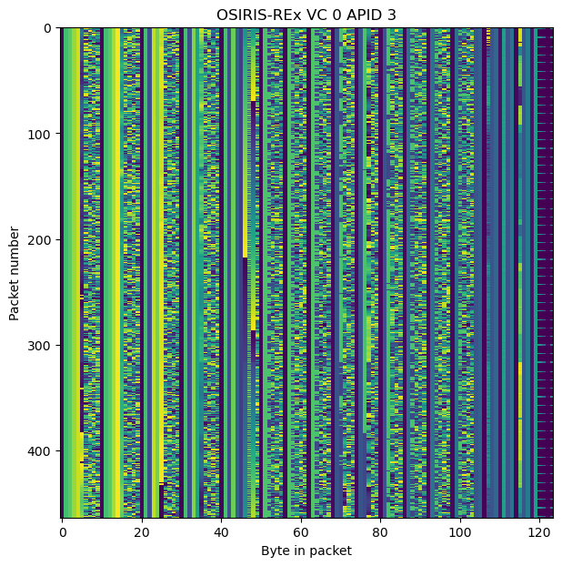
The raster map suggests the presence of floating-point fields, and indeed this is the case. Many of these fields are 64-bit or 32-bit floating point (always transmitted in big-endian format). The first 4 key-value fields are 64-bit floating point. They are attitude quaternions, since their squares add up to one.
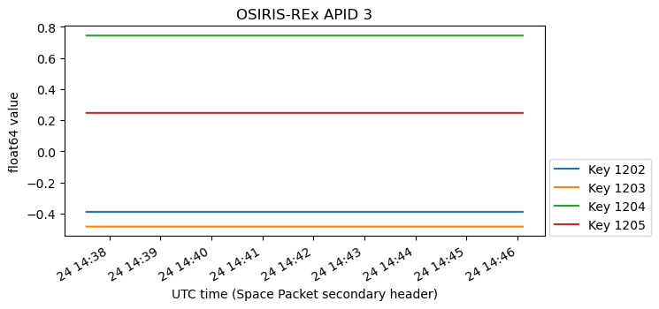
The attitude quaternions are almost constant, which indicates that the spacecraft attitude didn’t change significantly during the observation. In this post I have not analysed the spacecraft attitude, but it would be interesting to compare these quaternions with the SPICE kernels and with the received signal strength and spacecraft antenna pattern.
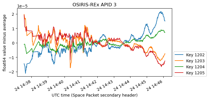
If we subtract its average to each of the quaternion components we can see some small variation during the observation.
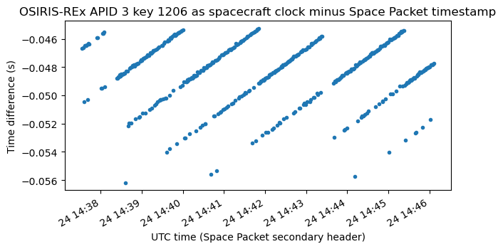
The next field is also 64-bit floating point. It contains spacecraft timestamps (as the number of seconds since the J2000 epoch). It is probably the timestamps associated to the attitude quaternions, and possibly other data in these packets. It is interesting to plot the difference between the timestamps in these field, and the timestamps in the Space Packet secondary header. These differences give (with a minus sign) the delay between the instant in which the attitude data is sampled, and the instant in which the data is put in a Space Packet.
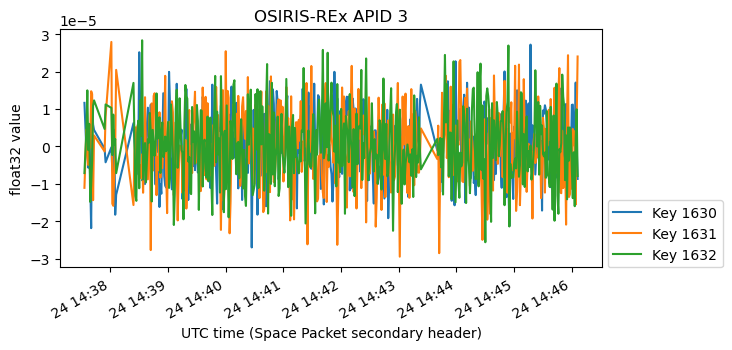
The next three fields are 32-bit floating point, and they contain a noise-like signal of small amplitude. I think that these are gyroscope values.
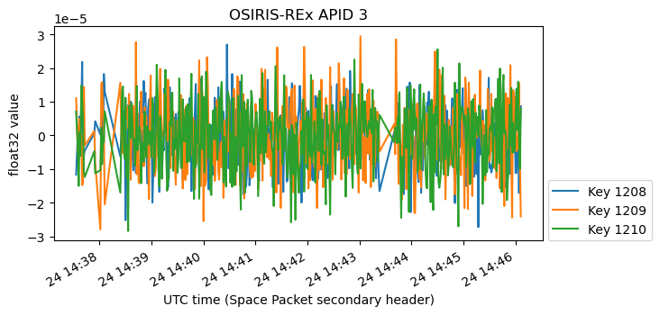
The following three fields are also 32-bit floating point and they contain some curves which look similar to the attitude quaternions minus their average. This suggests that they are angular errors.
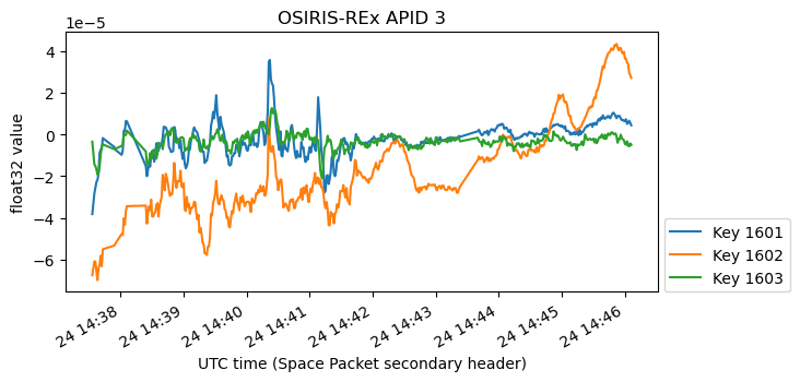
Next there is another set of three 32-bit floating point values which also seem to be gyroscope data (from another set of gyroscopes).
There are 5 more fields in the packets of APID 3 (including the extra field which is only present sometimes). There are plots of all of these in the Jupyter notebook, but none of them contain data that I can identify at a first glance.
In summary, it seems that APID 3 is dedicated to sending ADCS data at a rate of one measurement per second.
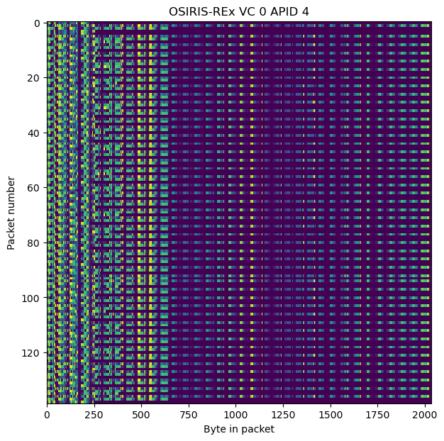
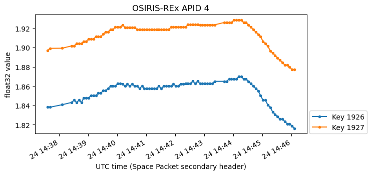
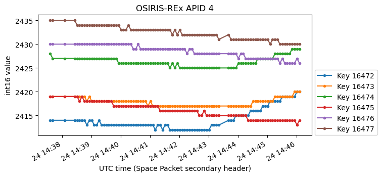
APID 4
The raster map for APID 4 is shown below. This shows packets reaching the maximum length and some short packets. The fields do not line up nicely anymore (though patterns can be seen), so using the key-value structure is necessary to parse this APID, which also happens in the other remaining APIDs.
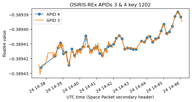
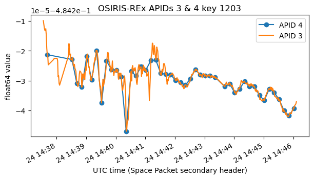
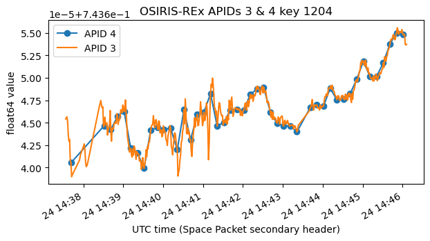
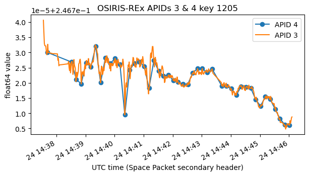
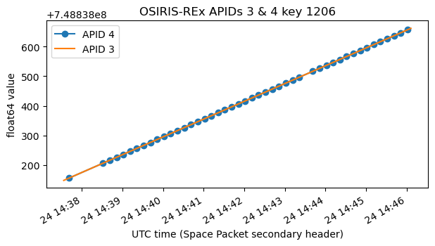
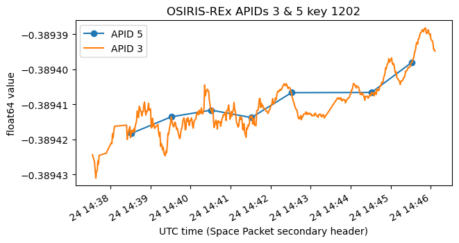
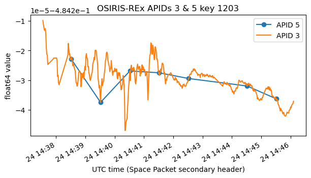
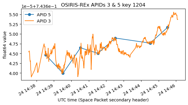
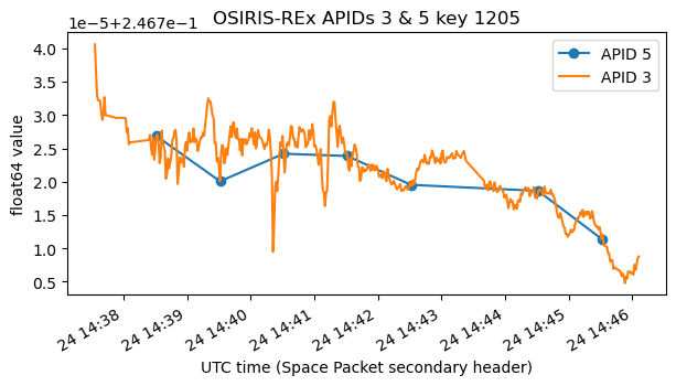
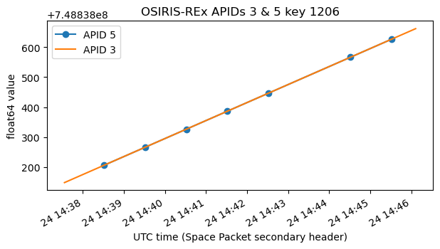
This APID contains keys 1202-1206, which correspond to the attitude quaternions in APID 3. Here they carry the same data, but sampled with a time resolution of one measurement every 10 seconds. The following figures show a comparison of the data corresponding to each of these keys in APID 3 and APID 4. The last key (key 1206) shows the raw timestamp values (which have units of seconds).
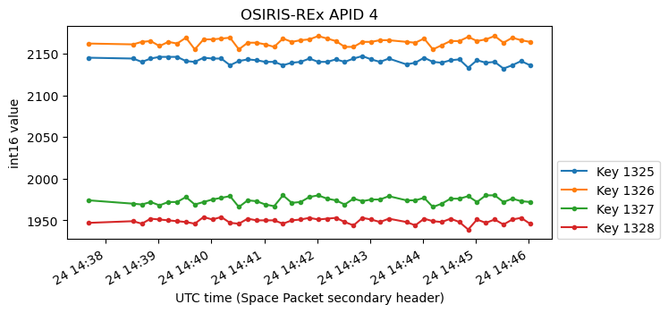
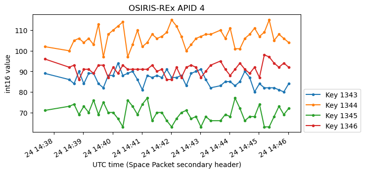
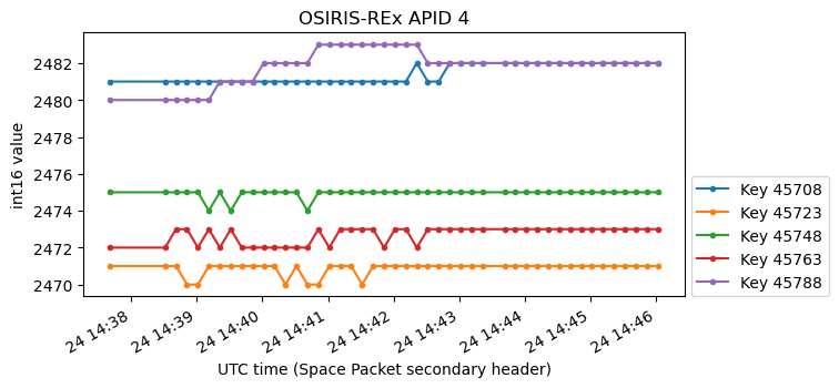
The next figures show a selection of other keys that I have found specially interesting in this APID (though I don’t know what they are). There are more plots in the Jupyter notebook. These plots also show that different keys have different reporting rates in APID 4.
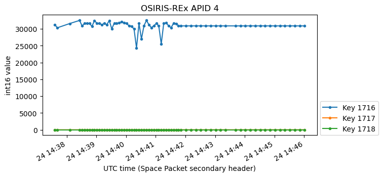
The following is specially interesting because it shows a change in reporting rate immediately before 14:42 UTC.
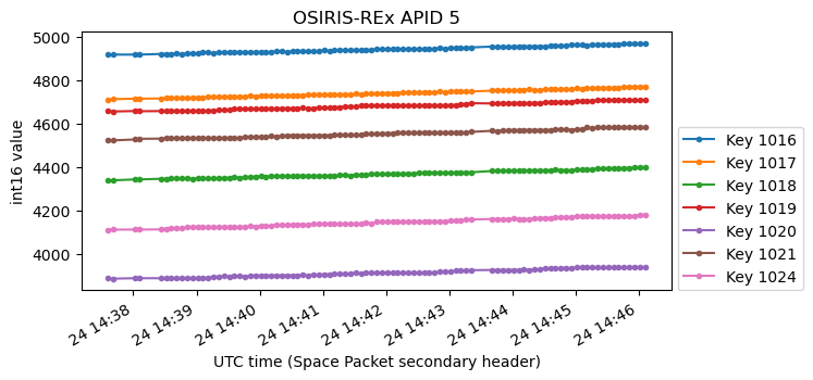
APID 5
APID 5 usually has short packets, but periodically there are two long packets sent in a row (one of them reaching maximum length). These correspond to the spikes for this APID in the plots of the packets per second and bytes per second. We can also see that at around packet number 50 the size of short packets gets smaller. As we will see, this happens because some of the keys start to be omitted from the short packets, and only appear in the long periodic bursts.
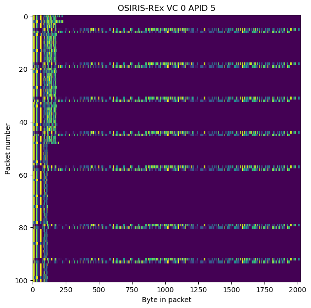
The long periodic bursts consist of many different APIDs. I have not looked at the contents of these, because it is quite difficult to figure out what a plot represents if there are only 7 data points.
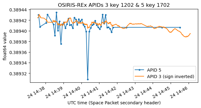
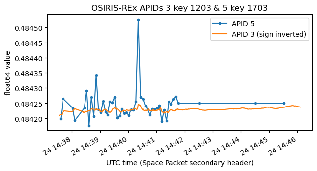
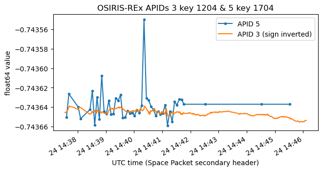
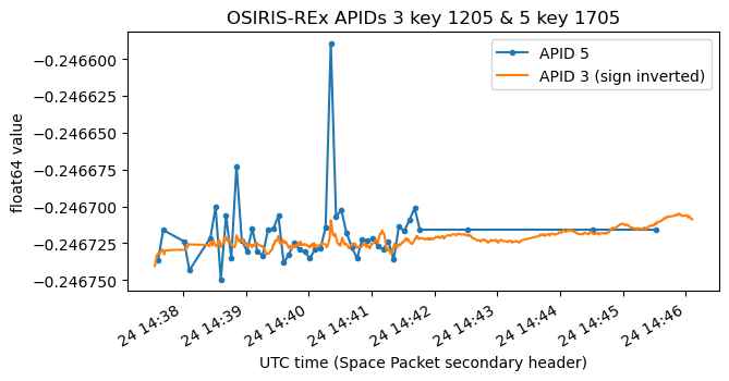
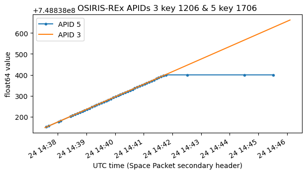
As in the case of APID 4, APID 5 also contains keys 1202-1206 with the attitude quaternions. These only appear in the periodic bursts, so they get reported once every 60 seconds. The following plots compare the data in APIDs 3 and 5 for these keys.
There is more quaternion data in APID 5. Keys 1702-1706 contain quaternion data in the same format as keys 1202-1206. However, this data seems to come from another ADCS source, because it is more noisy and the sign is inverted (remember that inverting the sign of a quaternion doesn’t change the rotation it represents). Initially, these quaternions are reported every 5 seconds, as they appear in the short Space Packets. Interestingly, shortly before 14:42 UTC, the values become frozen (including the timestamp) and are only reported every 60 seconds in the long packets. This corresponds to the change that we saw in the raster map for this APID and also in the packets per second and bytes per second plots. Since the spacecraft wasn’t being telecommanded during this observation, I think that the change was caused because of a pre-programmed command.
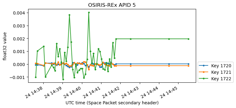
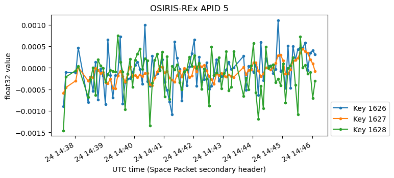
There are other keys in APID 5 that show the same change. For instance, keys 1720-1722. Perhaps they contain the angular errors.
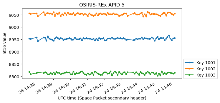
Here are some other interesting examples of keys in APID 5. These are always reported every 5 seconds.
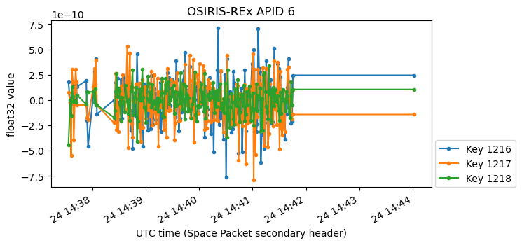
APID 6
APID 6 is similar to APID 5 in the sense that it usually transmits short packets, but every 150 seconds there is a long burst of maximum length packets. This burst corresponds to the 6.6 KB/s peaks in the bytes per second plot and is used to transmit a large number of different keys, most of which do not appear outside of these bursts. The bursts are the reason for the large number of different keys in this APID (a total of 12578 keys). I guess that these bursts are intended as a low rate way of reporting all the spacecraft telemetry channels. Interestingly, APID 6 does not have any keys in common with any of the other APIDs.
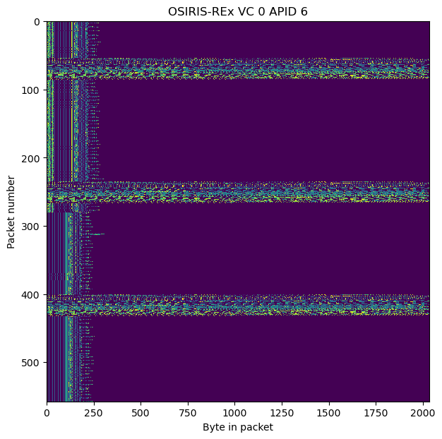
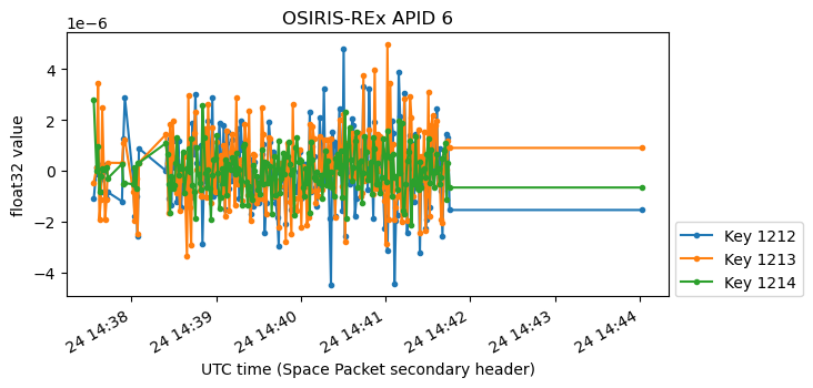
Halfway in the raster map we can also see the same kind of change as in APID 5. Some of the keys are removed from the short packets. The plots of some of these keys are shown below. The amplitude and noise-like aspect of them suggests that they are also gyroscope data (plus the number of their keys is also close to some of the APID 3 ADCS keys). It also seems that the values get frozen after 14:42 UTC, and they only appear in the bursts every 150 seconds.
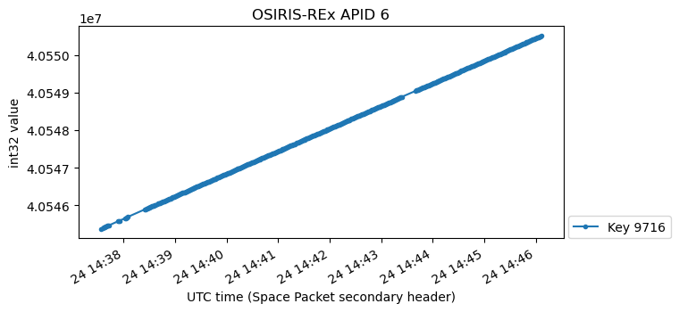
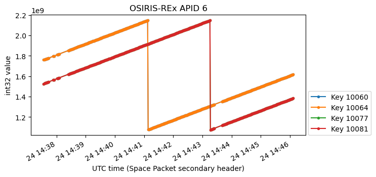
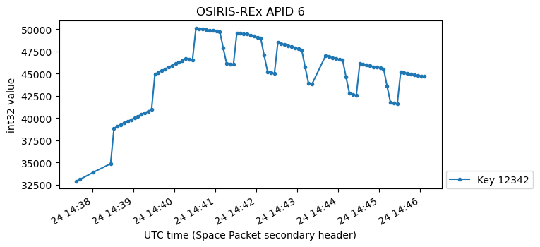
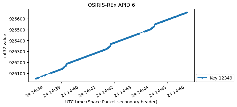
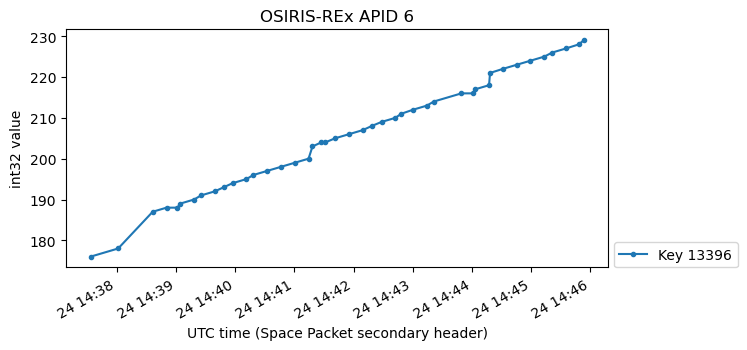
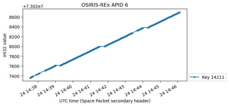
Some keys in this APID have 32-bit integer values (in big-endian format) and their values either increase linearly or have a sawtooth behaviour. The following two figures contain data reported every second.
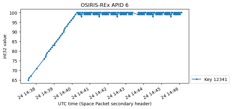
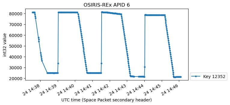
There are also some keys that are reported every 5 seconds, such as this one.

The Jupyter notebook contains more examples of these.
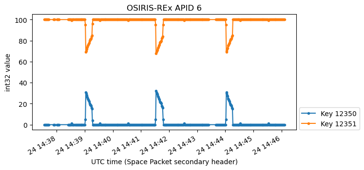
The following keys look interesting, and I have the impression that they are related, since the periods of the patterns they show match.
Summary of the telemetry
The telemetry of OSIRIS-REx received in this observation is distributed into APIDs 3, 4, 5, and 6. APID 3 seems completely or mostly dedicated to the ADCS, and includes quaternion, gyroscopes and angular errors data. It is the most regular APID, reporting all of the values except one at a rate of 1 second. The same quaternion data also appears in APIDs 4 and 5 at a lower reporting rate of 10 seconds and 60 seconds respectively. APIDs 5 and 6 have periodic bursts of packets every 60 seconds and 150 seconds which include many more values than those which are reported with more frequent periodicities. The bursts every 150 seconds in APID 6 are by far the largest. APID 5 and 6 seem to contain some ADCS data reporting every second, but it seems to come from a different source compared to the data in APID 3. This alternative ADCS data stops somewhat before 14:42 UTC, and the last values appear frozen in the bursts every 60 seconds or 150 seconds in each APID. APIDs 4, 5 and 6 contain different values reported at different intervals, typically either 1 second or 5 seconds, which gives irregularity to the structure of their packets.
Code and data
The Jupyter notebook used to prepare the antenna tracking using SPICE and to analyse the antenna tracking tests, the GNU Radio flowgraphs used to decimate the recording to 2.048 Msps and to compute the waterfall, and the Jupyter notebook used to plot the waterfall can be found in this repository.
The GNU Radio decoder, the binary file containing the decoded AOS frames, and the Jupyter notebook with the telmetry analysis are in this repository.
The IQ recordings are in the Zenodo dataset “Recording of OSIRIS-REx with the Allen Telescope Array during SRC reentry“. Only the recording for antenna 1a polarization X has been used in this post.
5 comments