This forms parts of a series of posts showing how to use GMAT to track the DSLWP-B Chinese lunar satellite. In part I we looked at how to examine and validate the tracking files published by BG2BHC using GMAT. It is an easy exercise to use GMAT to perform orbit propagation and produce new tracking files. However, note that the available tracking files come from orbit planning and simulation, not from actual measurements. It seems that the elliptical lunar orbit achieved by DSWLP-B is at least slightly different from the published data. We are already working on using Doppler measurements to perform orbit determination (stay tuned for more information).
Recall that there are three published tracking files that can be taken as a rough guideline of DSLWP-B’s actual trajectory. Each file covers 48 hours. The first file starts just after trans-lunar injection, and the second and third files already show the lunar orbit. Therefore, there is a gap in the story: how DSLWP-B reached the Moon.
There are at least two manoeuvres (or burns) needed to get from trans-lunar injection into lunar orbit. The first is a mid-course correction, whose goal is to correct slightly the path of the spacecraft to make it reach the desired point for lunar orbit injection, which is usually the lunar orbit periapsis (the periapsis is the lowest part of the elliptical orbit). The second is the lunar orbit injection, a braking manoeuvre to get the spacecraft into the desired lunar orbit and adjust the orbit apoapsis (the highest part of the orbit). Without a lunar orbit injection, the satellite simply swings by the Moon and doesn’t enter lunar orbit.
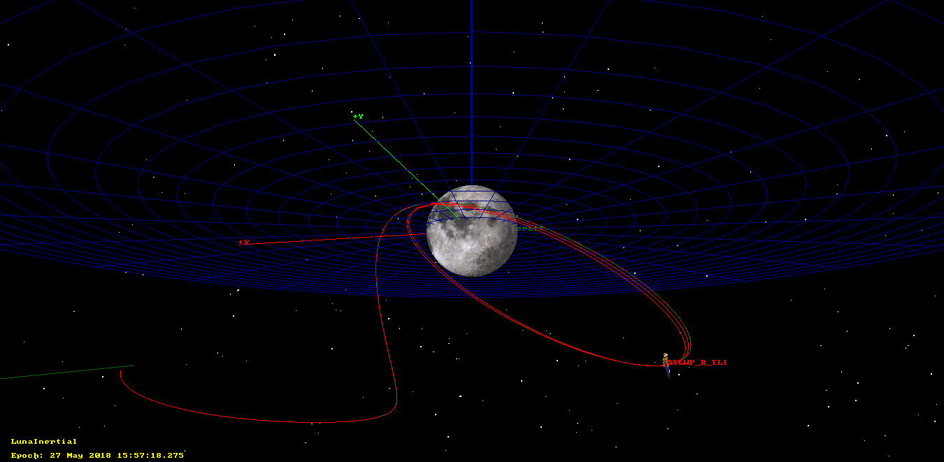
In this post we will see how to use GMAT to calculate and simulate these two burns, so as to obtain a full trajectory that is consistent with the published tracking files. The final trajectory can be seen in the figure below.