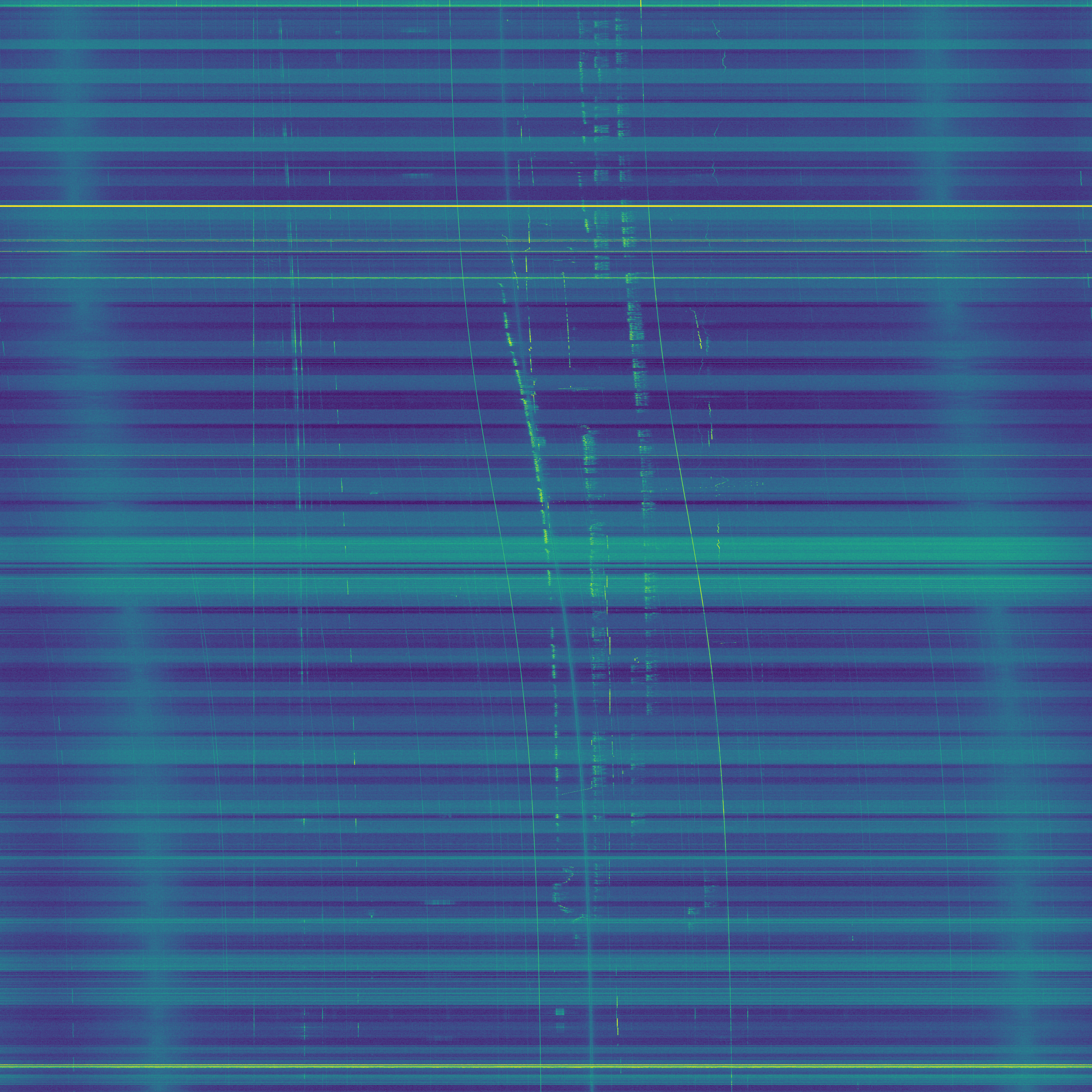
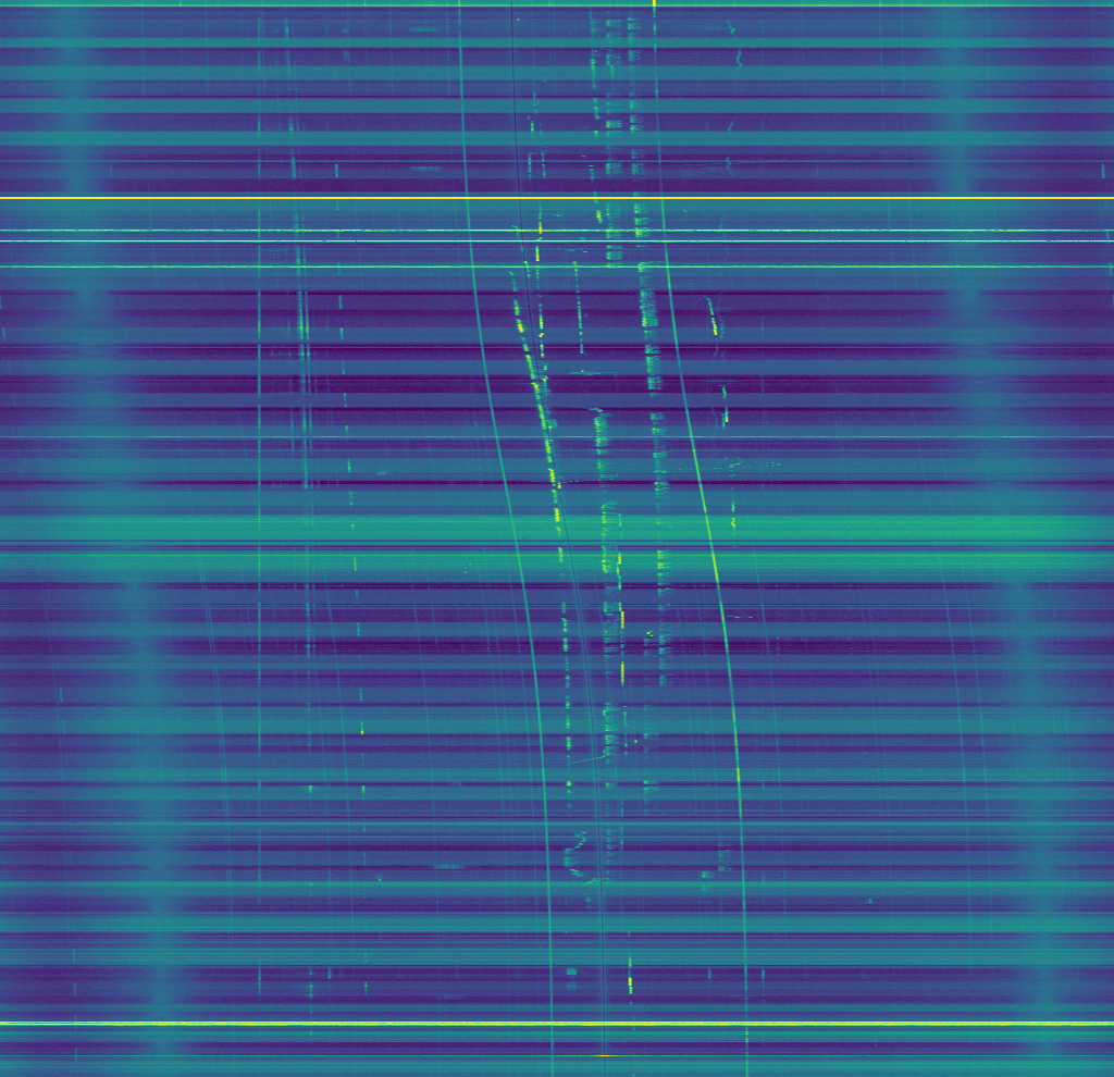
Over the last few days, I have been recording CODAR on 4463kHz to produce images of the ionosphere. I started on Friday 15th and the plan was to leave the recording running until Christmas Day, thus producing some kind of “CODAR advent” images. Unfortunately, there seems to be a problem when the receiver runs for several days that results in the sudden loss of the CODAR signal. This problem can be seen at the bottom of the image below. Thus, I have finished the recording on the morning of the 24th. The equipment and software used is the same that I detailed in a previous post.
Category: Experiments
Measurements, transmissions, receptions, etc. with the objective of obtaining and analysing some data.
Using CODAR for ionospheric sounding
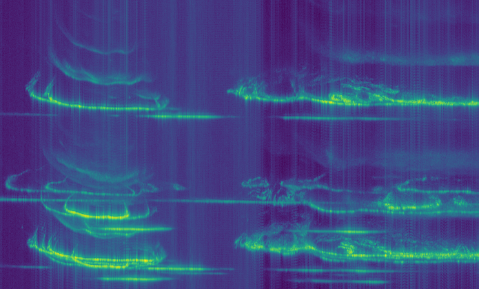
CODAR is an HF radar used to measure surface ocean currents in coastal areas. Usually, it consists of a chirp which repeats every second. The chirp rate is usually on the order of 10kHz/s, and the signal is gated in small pulses so that the CODAR receiver can listen between pulses. The gating frequency can be on the order of 1kHz.
CODAR can be received by skywave many kilometers inland. Being a chirped signal, it is easy to extract the multipath information from the received signal. In this way, one can see the signal bouncing off the different layers of the ionosphere, and magnificent pictures showing the changes in the ionosphere (especially at dawn and dusk) can be obtained. For instance, see these images by Pieter Ibelings N4IP, or the image at the top of this post, which contains 48 hours worth of CODAR data.
Here I describe my approach to receiving CODAR. It uses GNU Radio for most of the signal processing, and Python with NumPy, SciPy and Matplotlib for plotting.
A brief study of TLE variation
During my research and experiments about using WSJT-X modes through linear transponder satellites, one of the questions I had is by how much do TLEs of different epochs for the same satellite vary. This was glimpsed in part II, where I plotted the “best delay” parameter for TLEs of different age.
The topic of accuracy in TLE computation and propagation is rather complex. A NORAD TLE is the result of an orbit determination after several radar measurements at different epochs, so the elements are in some sense “averaged” over time. Also, the SGP4 propagator is simple and doesn’t model many orbit perturbations. However, NORAD TLEs are specially crafted to give improved results when used with SGP4.
Nevertheless, here I present a simple way of studying the rate of change of NORAD TLEs at different epochs. This procedure might not be very meaningful or sophisticate, but still seems to yield some interesting results.
Waterfall from the FT8 test through FO-29
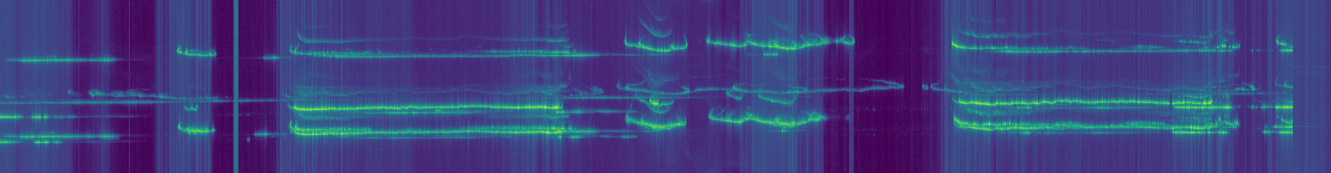
In the previous post, I detailed my experiments transmitting FT8 through the FO-29 linear transponder. I recorded a complete pass of the FO-29 satellite while I transmitted an FT8 signal trough the transponder on even periods. As I promised in that post, I have now made a waterfall with the recording to show the activity through the linear transponder, and the strength of my FT8 signal in comparison with the SSB and CW signals of other users.
The watefall can be seen below. You can click on the image to view it in full size. A higher resolution version is available here (24MB). The horizontal axis represents frequency and the vertical axis represents time, with the beginning of the pass at the top of the image. The waterfall has been corrected for the downlink Doppler and the DC spike of the FUNcube Dongle Pro+ has been removed.
From left to right, the following signals can be seen: The CW beacon can be seen as a faint vertical signal. Next, there is some interference coming through the transponder in the form of terrestrial FM signals. Then we can see my FT8 signal, being transmitted only on even periods. Finally, around the centre of the image, we have a few SSB and CW signals through the transponder. Note that most of these signals increase in frequency as the pass progresses. This is because many people keep a fixed uplink and only tune the downlink by hand to correct for Doppler. Unfortunately, full computer Doppler correction is not very popular. I also used a fixed uplink frequency for my FT8 signal, but only to simplify the experiment. The best procedure is to correct for the uplink Doppler to keep a constant frequency at the satellite.
We can see that the SSB and CW signals are much stronger than my FT8 signal. Indeed, some of the CW signals are particularly strong at times, perhaps putting too much pressure on the linear transponder.
The waterfalls in this post have been created using this Jupyter notebook.
First FT8 test through FO-29
Continuing with my research on using WSJT-X modes through linear transponder satellites in low Earth orbit (see part I and part II), a few days ago I transmitted and recorded an FT8 signal through the V/U linear transponder on FO-29 during a complete pass. The recording started at 2017/10/23 20:26:00 UTC and ended at 20:42:30 UTC. It was made with a FUNcube Dongle Pro+ set to a centre frequency of 435.850MHz and connected to a handheld Arrow satellite yagi through a duplexer. Here the duplexer was used to avoid desense on transmit.
An FT8 signal was transmitted on every even period during the recording, at a fixed frequency of 145.990MHz, using a Yaesu FT-817ND and the Arrow antenna. The signal was transmitted using lower sideband (i.e., inverted in the frequency domain) to get a correct FT8 signal through the inverting transponder. The transmit power was adjusted often to get a reasonable signal through the transponder and avoid using excessive power. There have been reports and complaints of people using too much power with digital modes through linear satellites. In this post, a study of the power is included to show that it is possible to use digital modes effectively without putting any pressure on the satellite’s transponder.
Out of the 33 even periods, a total of 24 can be decoded by WSJT-X using the best TLEs from Space-Track. No measures were taken to correct for the time offset \(\delta\) that has been studied in the previous posts, as the TLEs already provided a good Doppler correction. Regarding the choice of TLEs, there are still some remarks to make. First, the epoch of the TLEs used was 2017/10/23 21:39:16 UTC, so these TLEs were actually taken after the pass. The previous TLEs were taken a few hours before the pass, and it is likely that they also provided a good correction, perhaps by using a time offset \(\delta\) if necessary. However, I do not know if these previous TLEs were also available from CelesTrak before the start of the pass, as it seems that TLEs take a while to propagate from Space-Track to Celestrack. To explain why the TLEs with no time offset correction are enough, it will be interesting to study the rate of change of TLE parameters for FO-29. This will be done in a future post.
The results of this test look very promising. Even though this wasn’t an overhead pass (the maximum elevation was 40º), the maximum rate of change of the Doppler was over 20Hz/s for the self-Doppler seen on the FT8 signal and 35Hz/s for the downlink Doppler seen on the CW beacon. Most of the periods which couldn’t be decoded were near the start or end of the pass. This is the only test that I know of that has decoded FT8 signals in the presence of high rates of change of Doppler. The previous tests by other people were made at low elevations, where the rate of change of Doppler is small. This test has shown that it is possible to get many decodes with high rates of change of Doppler, even using no corrections to the TLEs. Here I continue with a detailed analysis of the recording.
WSJT-X and linear satellites: part II
This is a follow-up to the part I post about using WSJT-X modes through a linear transponder on a LEO satellite. In part I, we considered the tolerance of several WSJT-X modes to the residual Doppler produced by a temporal offset in the Doppler computation used for computer Doppler correction. There, we introduced a parameter \(\delta\) which represents the time shift between the real Doppler curve and the computed Doppler curve. The main idea was that a decoder could try to correct the residual Doppler by trying several values of \(\delta\) until a decode is produced.
Here we examine the effect of TLE age on the accuracy of the Doppler computation. The problem is that, when a satellite pass occurs, TLEs have been calculated at an epoch in the past, so there is an error between the actual Doppler curve and the Doppler curve predicted by the TLEs. We show that the actual Doppler curve is very well approximated by applying a time shift to the Doppler curve predicted by the TLEs, justifying the study in part I.
Measuring a mains choke with Hermes-Lite VNA
I have made a mains choke for my HF station, following Ian GM3SEK’s design, which involves twisting the three mains wires together and passing as many turns as possible through a Fair-Rite 0431177081 snap-on ferrite core. I wanted to measure the choke’s impedance to get an idea of its performance, so I’ve used my Hermes-Lite 2.0 beta2 in VNA mode.
Polarization in Voyager signal from Green Bank Telescope
A few days ago I read the paper about the Breakthrough Listen experiment. This experiment consists in doing many wideband recordings of different stars using the Green Bank Telescope, and (in the future) Parkes Observatory and then trying to find signals from extraterrestrial intelligent life in the recordings. The Breakthrough Listen project has a nice Github repository with some documentation and an analysis of a recording they did of Voyager 1 to test their setup.
I have also been thinking about how to study the polarization of signals in a dual polarization recording (two coherent channels with orthogonal polarizations). My main goal for this is to study the polarization of the signals of Amateur satellites in low Earth orbit. It seems that there are many myths regarding polarization and the rotation of cubesats, and these myths eventually pop up whenever anyone tries to discuss whether linearly polarized or circularly polarized Yagis are any good for receiving cubesats.
Through the Breakthrough Listen paper I’ve learned of the Stokes parameters. These are a set of parameters to describe polarization which are very popular in optics, since they are easy to measure physically. I have immediately noticed that they are also easy to compute from a dual polarization recording. In comparison with Jones vectors, Stokes parameters disregard all the information about phase, but instead they are computed from the averaged power in different polarizations. This makes their computation less affected by noise and other factors.
As I also wanted to get my hands on the Breakthrough Listen raw recordings, I have been computing the Stokes parameters of the Voyager 1 signal in their recording. Since the Voyager 1 signal is left hand circularly polarized, the results are not particularly interesting. It would be better to use a signal with changing polarization or some form of elliptical polarization.
I have started to use Jupyter notebook. This is something I had been wanting to try since a while ago, and I’ve realised that a Jupyter notebook serves better to document my experiments in Python than a Python script in a gist, which is what I was doing before. I have started a Github repo for my experiments using Jupyter notebooks. The experiment about polarization in the Voyager 1 signal is the first of them. Incidentally, this experiment has been done near Voyager 1’s 40th anniversary.
WSPR reports frequency distribution experiment: 20m
Last week I did an experiment where I transmitted WSPR on a fixed frequency for several days and studied the distribution of the frequency reports I got in the WSPR Database. This can be used to study the frequency accuracy of the reporters’ receivers.
I was surprised to find that the distribution of reports was skewed. It was more likely for the reference of a reporter to be low in frequency than to be high in frequency. The experiment was done in the 40m band. Now I have repeated the same experiment in the 20m band, obtaining similar results.
AGC for gr-satellites
In a previous post I discussed my BER simulations with the LilacSat-1 receiver in gr-satellites. I found out that the “Feed Forward AGC” block was not performing well and causing a considerable loss in performance. David Rowe remarked that an AGC should not be necessary in a PSK modem, since PSK is not sensitive to amplitude. While this is true, several of the GNU Radio blocks that I’m using in my BPSK receiver are indeed sensitive to amplitude, so an AGC must be used with them. Here I look at these blocks and I explain the new AGC that I’m now using in gr-satellites.