In my previous post I spoke about the recording I made of the X-band telemetry signal of Hera with the Allen Telescope Array shortly after it was launched. Despite the lack of publicly available accurate ephemerides at the time of launch, I managed to track the spacecraft by hand and decode a good amount of telemetry frames. In this post I will do an in-depth analysis of the telemetry.
Author: destevez
Decoding Hera
Hera is an ESA mission to the Didymos binary asteroid system. It will arrive there in December 2026 to study the asteroids and the effects of the impact of DART on Dimorphos. It was launched on October 7 from Cape Canaveral, exactly one week before Europa Clipper. In the same way as for Europa Clipper, Hera’s launch trajectory allowed me to track it with the Allen Telescope Array, starting approximately 90 minutes after launch.
However, the ephemerides publicly available when the launch happened turned out to be completely wrong, as I will explain below in more detail. I needed to find the spacecraft’s signal by moving the antenna in the blind, and continue tracking it by hand by tweaking the pointing every few minutes. For this reason, the quality of the recordings I have done is not so good. The signal drops down frequently as the spacecraft moves away from where I was pointing or when I made mistakes in my pointing adjustments.
For this reason, I have prioritized decoding the Europa Clipper recordings, since I expected that decoding these low quality recordings of Hera would take more work. Nevertheless I have managed to decode a good amount of telemetry.
I have published the IQ recordings made with the ATA in the following two Zenodo datasets:
Europa Clipper telemetry
In my previous post I spoke about the recording I did of the Europa Clipper X-band telemetry shortly after launch with one of the Allen Telescope Array antennas. In that post I analysed the recording waterfall and the signal modulation and coding, and decoded the telemetry frames with GNU Radio. In this post I analyse the contents of the telemetry. As we will see, there are several similarities with the telemetry of Psyche. This makes sense, because both are NASA missions that have been launched only one year apart.
Decoding Europa Clipper
Europa Clipper is a NASA mission that will study Europa, Jupiter’s icy moon, to investigate if it can support life, perhaps in hydrothermal vents in a global ocean under the ice crust. The mission launched on Monday from Cape Canaveral, after some days of delay due to Hurricane Milton. As happened with Psyche one year ago, the launch trajectory was such that the first pass over the Allen Telescope Array, in northern California, started only about 1.5 hours after launch. To put this in perspective, launch was at 2024-10-14T16:06 UTC, spacecraft separation at T+1:02:39, and my recording began at 17:33:24 UTC, with signal acquisition a couple minutes later as the spacecraft raised above the 16.8 deg elevation mask of the ATA antennas.
I used one of the ATA antennas to record the X-band telemetry signal for about 2 hours and 50 minutes, until the spacecraft set again due to Earth rotation. In this post I overview the recording and decode the telemetry with GNU Radio.
I recorded at 6.144 Msps IQ, but since the telemetry symbol rate was only 12 kbaud throughout all the recording, I have made files decimated to 96 ksps and published them in the dataset “Recording of Europa Clipper X-band telemetry with the Allen Telescope Array shortly after launch” in Zenodo. This decimation discards the sequential ranging tones, which were present during most of the observation, but it greatly reduces the file size.
Analysis of DME signals
You might remember that back in July I made a recording of the DME ground-to-air and air-to-ground frequencies for a nearby VOR-DME station. In that post, I performed a preliminary analysis of the recording. I mentioned that I was interested in measuring the delay between the signals received directly from the aircraft and the ground transponder replies, and match these to the aircraft trajectories. This post is focused on that kind of study. I will present a GNU Radio out-of-tree module gr-dme that I have written to detect and measure DME pulses, and show a Jupyter notebook where I match aircraft pulses with their corresponding ground transponder replies and compare the delays to those calculated from the aircraft positions given in ADS-B data.
Not-LoRa GRCon24 CTF challenge
This year I submitted a track of challenges called “Not-LoRa” to the GRCon 2024 Capture The Flag. The idea driving this challenge was to take some analog voice signals and apply chirp spread spectrum modulation to them. Solving the challenge would require the participants to identify the chirp parameters and dechirp the signal. This idea also provided the possibility of hiding weak signals that are below the noise floor until they are dechirped, which is a good way to add harder flags. This blog post is an in-depth explanation of the challenge. I have put the materials for this challenge in this Github repository.
To give participants a context they might already be familiar with, I took the chirp spread spectrum parameters from several common LoRa modulations. These ended up being 125 kHz SF9, SF11 and SF7. LoRa is somewhat popular within the open source SDR community, and often there are LoRa challenges or talks in GRCon. This year was no exception, with a Meshtastic packet in the Signal Identification 7 challenge, and talks about gr-lora_sdr and Meshtastic_SDR.
Testing gr4-packet-modem through a GEO transponder
During the last few months, I have been working on gr4-packet-modem. This is a packet-based QPSK modem that I’m writing from scratch using the GNU Radio 4.0 runtime. The gr4-packet-modem project is funded by GNU Radio with an ARDC grant, and its goal is to produce a complete digital communications application in GNU Radio 4.0 that can serve to test how well the new runtime works in this context and also as a set of examples for people getting into GNU Radio 4.0 development. I have presented gr4-packet-modem in the EU GNU Radio days (see the recording in YouTube).
In July, Frank Zeppenfeldt, who works in the satellite communications group in ESA, got in touch with me regarding an opportunity to test gr4-packet-modem on a C-band transponder on Intelsat 37e. His group is running a project with industry about a test campaign of IoT communications over GEO satellites, and they have rented a 1 MHz C-band transponder on Intelsat 37e for some time. The uplink is somewhere around 5.9 GHz, and the downlink somewhere around 3.7 GHz. As part of the project, they have setup a PC and a USRP B200mini in a teleport in Germany that has a large antenna to receive the downlink. There is remote access to this PC, so all the downlink part of the experiments is taken care of: IQ recordings can be made and receiver software can be run in this PC. Therefore, if I could set up an uplink station at home in Madrid (which is actually slightly outside the edge of the Europe C-band beam, as it can be seen in this document), then I would be able to run some tests of gr4-packet-modem by running the transmitter in my laptop and the receiver in the remote PC at the teleport.
As I mentioned to Frank when he proposed this experiment, I haven’t implemented an FEC for the payload of the packets in gr4-packet-modem, because I wanted to have full freedom in setting the size of each packet (to test latency with different packet sizes), and a good FEC scheme usually constraints the possible packet sizes (see gr-packet-modem waveform design for more details). Testing a modem that uses uncoded QPSK over a GEO channel is somewhat pointless, but Frank and I agreed that this would be a fun experiment, even if not too interesting from the technical point of view. In the rest of the post I explain the test set up and results.
JUICE Earth flyby
At the beginning of this week, JUICE, an ESA spacecraft that was launched in April 2023 and that will explore Jupiter’s icy moon, completed its lunar-Earth flyby. This is the first time that such a manoeuvre has been done. I’m far from an expert in orbital dynamics, but I hear that by doing a combined lunar-Earth flyby instead of the more traditional Earth flyby there can be delta-V savings for the mission. The IAC paper Improved interplanetary transfers with Lunar-Earth gravity assists seems to be the first that presented this idea, but I haven’t found the paper itself. The JUICE mission analysis report (CReMA) contains some more information, but it is not too detailed and somewhat outdated. Perhaps a good source to learn about this is a master’s thesis called Automatic extension of Earth and Earth-Moon resonant flybys, although I’ve only had time to read a small part of it.
The following image that I made in GMAT with the mission SPICE kernels illustrates the geometry of the flybys. The lunar flyby happened on 2024-08-19 21:15 UTC, and the Earth flyby happened on 2024-08-20 21:56 UTC.
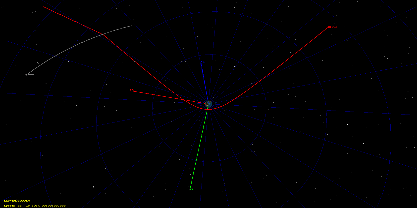
The Earth flyby happened 6840 km above the north Pacific ocean, so the spacecraft was visible from the Allen Telescope Array, in northern California, starting some minutes after the flyby. I thus decided to observe JUICE with one of the 6.1 m dishes of the array and record its X-band telemetry signal roughly between 22:00 and 23:00 UTC. That would be a fun way of “saying hello” again to the spacecraft (see the post where I recorded and decoded its telemetry when it launched in April last year).
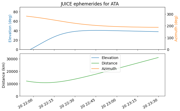
I prepared a tracking file for antenna pointing in the same way that I did for the OSIRIS-REx flyby during its sample capsule return. I used the SPICE kernels to compute a time series of azimuth and elevations for the antenna. For the spacecraft orbit I used the juice_orbc_000071_230414_310721_v01.bsp SPICE kernel, which was the latest available at the time. This kernel was created on 2024-08-15. The following plot shows the antenna azimuth and elevation and the distance to the spacecraft.
When I was about to begin observing, I saw a tweet from ESA Operations. Strangely the tweet has now been deleted. I hate it when information I once saw suddenly vanishes out of existence. I have the link to the tweet, but not a copy of it. It roughly said something along the lines of: “since JUICE is prepared for the cold thermal environment of Jupiter, to prevent it from overheating during the Earth flyby, data will not be transmitted to Earth until 2024-08-21 04:30 UTC”.
A problem with outreach communications is that they’re often vague with the hopes of simplifying to reach a wider audience. In this case, the context for the tweet was that ESA had run a livestream during the lunar flyby where they transmitted and showed images of the Moon in near-realtime. Postprocessed images with better quality were then released the next morning (see also this and related toots from Mark McCaughrean, who is one of the two persons responsible for the images). I think there was some word in social media that shortly after the Earth flyby some images would be shown, so the tweet served as a heads up that any images would need to wait until the next morning.
What wasn’t clear about the tweet is what this really meant about the spacecraft telemetry signal. Anyone familiar with spacecraft tracking will imagine that during the flyby there will be no groundstation coverage, because deep space stations can’t track that fast and probably won’t have the spacecraft in view. Therefore it’s clear that no images can be downloaded for some time around the flyby. But what about the telemetry signal? Does the tweet mean that there will be no housekeeping telemetry (which typically is sent all the time) either? Even no RF modulation at all? This might well be the case, especially since the tweet mentioned thermal reasons. If there isn’t going to be groundstation coverage for a while, why run the radio transmitter and generate more heat? But the way that the tweet was worded still made me doubt (I think the literal words were “it won’t transmit any more data”, but I don’t have the full sentence).
So after seeing that I wasn’t receiving any signal with the Allen Telescope Array, I wasn’t too surprised. I tweeted about this, as a quote tweet (repost) of the ESA Operations tweet.
I finished recording data at 22:30 UTC, since by then I was convinced that the transmitter was off and there was no point in continuing to record. I ran some additional tests to rule out a problem with the receiver. Unfortunately there were no good deep space X-band satellites in view at that time, since Mars was just setting. I tried with Parker Solar Probe, which was being tracked by Goldstone, but I didn’t know its frequency and didn’t have an estimate for how strong the signal should be. I didn’t see the signal. I also tried with ACE, which transmits at S-band and was also tracked by Goldstone. I could receive it just fine, so I don’t have much reason to suspect about the receiver.
Another potential reason why no signal could be detected is if there was an error in the ephemerides that caused a large enough antenna pointing error. I don’t think this was the case, even though the ephemerides were not updated after the lunar flyby. To make sure, I will rerun the pointing calculations with the next SPICE kernel that gets published and compare them. Pointing error is also the reason that I kept recording until 22:30 UTC. The effect of ephemerides error in pointing error would become smaller as the distance to the spacecraft increased with time.
Just in case there was a faint signal, I have processed the recording to compute a waterfall with a resolution of 93.75 Hz and 10 seconds. The following two plots definitely show that there is no signal.
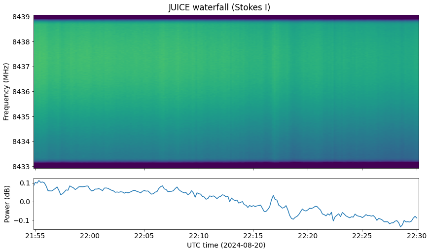
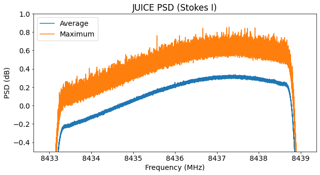
So with this, I finish the post as a failed observation of JUICE. I’ve decided do this write up because I think that, in science, negative results can be as important as positive results. In this case, the observation provides good evidence (especially now that the ESA Operations tweet is misteriously gone) that JUICE had the RF transmitter turned off during the Earth flyby. This is nothing transcendental, but rather an interesting tidbit of spacecraft operations trivia. The lack to detect any signals also reminds me of many astronomical observations, particularly those done as a followup to some transient, where if no signal is detected, the conclusion is often stated as “we establish upper bounds for the flux radiated by this source”.
To close with something more positive, I’ll mention that Alan Antoine F4LAU had a much more successful time tracking the lunar flyby with the AMSAT-DL 20 m antenna at Bochum Observatory, and he even found and decoded many images transmitted in the telemetry.
The materials used in this post can be found in this repository.
Final update for the Galileo GST-UTC anomaly
In September and October last year I was covering an anomaly with the Galileo GST-UTC offset (see also the update). I planned to keep posting updates as the event progressed, or at least once it was over, but I soon got distracted with other things, and this event didn’t get enough media coverage that would serve me as a reminder.
As a quick reminder, the Galileo GNSS maintains a timescale known as GST. This timescale is usually within a few nanoseconds of UTC, as is also the case for GPS time (although both GNSS systems give much larger margins when defining how much their timescales can deviate from UTC). In the beginning of September 2023, the GST-UTC offset reached a value of around 20 ns, much larger than it usually is. This surprised some people in the GNSS community, and I don’t recall there being a public explanation about what had happened.
Now this event is well past, so I can update my plots to show it in its full duration. For more details, refer to the first post. For this post I have used data ranging from 2023-07-16 to 2024-01-20. As in the previous posts, the data I’m using is the precise clock solution from CODE (the final products) and the broadcast ephemerides from IGS.
The difference between the broadcast ephemerides clock bias and the CODE precise clock bias is shown here. This quantity is a proxy for the GST-GPST offset, because CODE refers the timescale for its precise solutions to GPST. Since GPST is within a few ns of UTC, this is a good approximation for the GST-UTC offset.
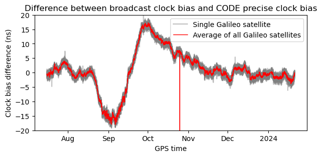
There is a glitch in the data sometime in October. I haven’t investigated this, and we can safely ignored it. We can see that the GST-UTC reaches nearly -20 ns in the beginning of September, then swings in the opposite direction, reaching almost 20 ns in the beginning of October, and then it takes all October and part of November before resuming usual levels around zero. I have included some data before August to show how the offset behaved before the anomaly began. It is clear that the behaviour in July and December is similar, so we can say that the system was restored mid-November.
The second plot I had was a comparison of the three offsets that are included in the broadcast ephemerides (GST-UTC, GPST-UTC, and GST-UTC) with the curve obtained above as the average of all Galileo satellites (with the sign flipped, due to sign conventions in the biases).
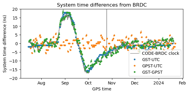
Besides the fact that the broadcast GST-UTC and GST-GPST biases follow quite closely the curve of the CODE-BRDC clock, there are other details that are quite apparent in this long term plot.
The first is that the GPST-UTC is quite noisy. Note that this isn’t part of Galileo. It is transmitted by the GPS constellation. It also seems that there is a positive correlation between the sign of the GPST-UTC and the sign of its derivative (the derivative is represented by a short slanted line crossing the point in question). Certainly, if we subtract the GST-UTC and GST-GPST offsets provided by Galileo, we obtain something much smaller than what GPS broadcasts as GPST-UTC.
The second is that the GST-UTC offset is sometimes held constant for periods of several weeks. In comparison, the GST-GPST varies more quickly. This makes sense, because measuring GST-UTC requires processing data from stations that are equipped with a Galileo timing receiver and that also have traceability to UTC, while measuring GST-GPST is something that any GNSS receiver can do with the ephemerides of both systems and observations of satellites in the two constellations.
I have updated the Jupyter notebook and the data used for this post in the repository.
2024’s update of Tianwen-1’s remote sensing orbit
Last year I wrote a post on July 23, which is the anniversary of Tiawen-1‘s launch. The post was essentially an updated plot of the orbital parameters of Tianwen-1’s remote sensing orbit. As I explained in that post, AMSAT-DL is using the 20 meter antenna in Bochum observatory to receive telemetry from Tianwen-1 almost every day (this can be followed in the YouTube livestream). Since Tianwen-1 includes its state vector (position and velocity with respect to Mars) in its telemetry, this allows us to monitor its orbit, which is of interest because no other public detailed information is available.
This year I completely forgot to do the same again for July 23, but I have remembered now. Here is the updated plot of the orbital parameters of Tianwen-1 since 8 November 2021, when the remote sensing orbit began. The plot includes data until 2 August 2024. During most of August, AMSAT-DL is not tracking Tianwen-1, since Mars has a very similar right ascension to STEREO-A, and tracking STEREO-A has priority. Tracking of Tianwen-1 will resume as the two objects drift apart in right ascension.
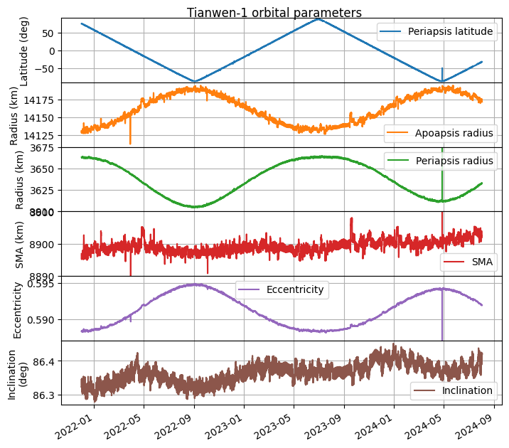
All the changes in the orbital parameters are due to perturbations by the Sun’s gravity and the oblateness of Mars, since as far as I know there have been no manoeuvres in this orbit. The main change in orbital parameters is a steady change in the latitude of the periapsis. The orbit is designed on purpose to exploit this effect. Over time, all the surface of Mars can be observed from a low altitude. This perturbation is related to a change in eccentricity, which is minimal when the periapsis is over the north pole and maximal when the periapsis is over the south pole.
Now it is quite apparent that there is also a slow but steady increase in inclination. This was not so evident last year, due to a sinusoidal perturbation that is also present, but now it is clear that the inclination has increased by about 0.05 deg since November 2021. It seems that this increase in inclination is related to a small increase in the semi-major axis.
The code for the updated plot can be found in this Jupyter notebook.