Hakuto-R Mission 1 is a private lunar mission led by the Japanese company ispace. It consists of a lander, which carries the Emirates Lunar Mission rover Rashid and JAXA/Tomy’s SORA-Q toy-like robot. It was launched on a Falcon 9 from Cape Canaveral together with the cubesat Lunar Flashlight on 11 December 2022, and will attempt to land on the Moon approximately 4.5 months after launch.
AMSAT-DL made some recordings of Lunar Flashlight and Hakuto-R M1 in the days following the launch using the 20 meter antenna at Bochum observatory. Here I will look at two recordings of the X-band telemetry signal of Hakuto-R M1 at 8492.5 MHz done on 2022-12-11 at 22:48:43 (121 seconds at 1.25 Msps IQ) and 23:23:08 UTC (54 seconds at 5 Msps IQ).
Modulation and coding
The modulation is PCM/PSK/PM with a symbol rate of 16 kbaud. The subcarrier frequency is supposed to be 8 times the symbol rate, but I’ve found that it is closer to 128.515 kHz. I have the impression that the symbol clock and subcarrier clock are not coherent, as happened with Tianwen-1, but I haven’t checked this. Coding is CCSDS Turbo coding with r=1/2 and 1115 byte frames in both recordings.
We have seen this choice of symbol rates and subcarrier frequencies which are powers of two in other Japanese spacecraft such as EQUULEUS, and in Chinese spacecraft such as Tianwen-1 and Chang’e 5. However, in those cases the frame size for concatenated coding was chosen in such a way that the coded frame length was a power of two. This caused the frame duration to be a power of two times one second. This is not possible in the case of Turbo coding, because the possible frame sizes are fixed, due to the design of the interleaver, and do not give power of two sizes.
In both recordings there is telecommand feed-through on the transponder. The telecommand signal uses a subcarrier of 16 kHz, and a symbol rate of 1 kbaud. There are two telecommands being sent in each of the recordings.
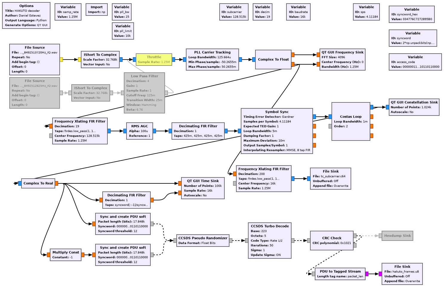
The figure below shows the GNU Radio flowgraph that I have used to decode both recordings. It uses the Turbo decoder block from gr-dslwp.
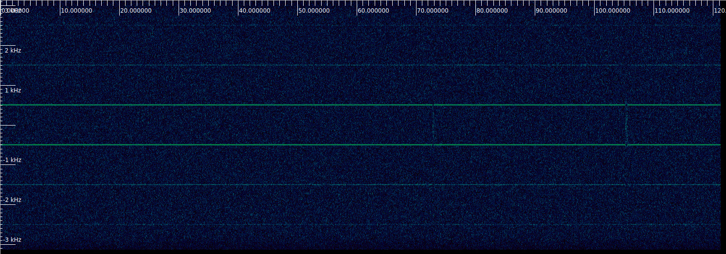
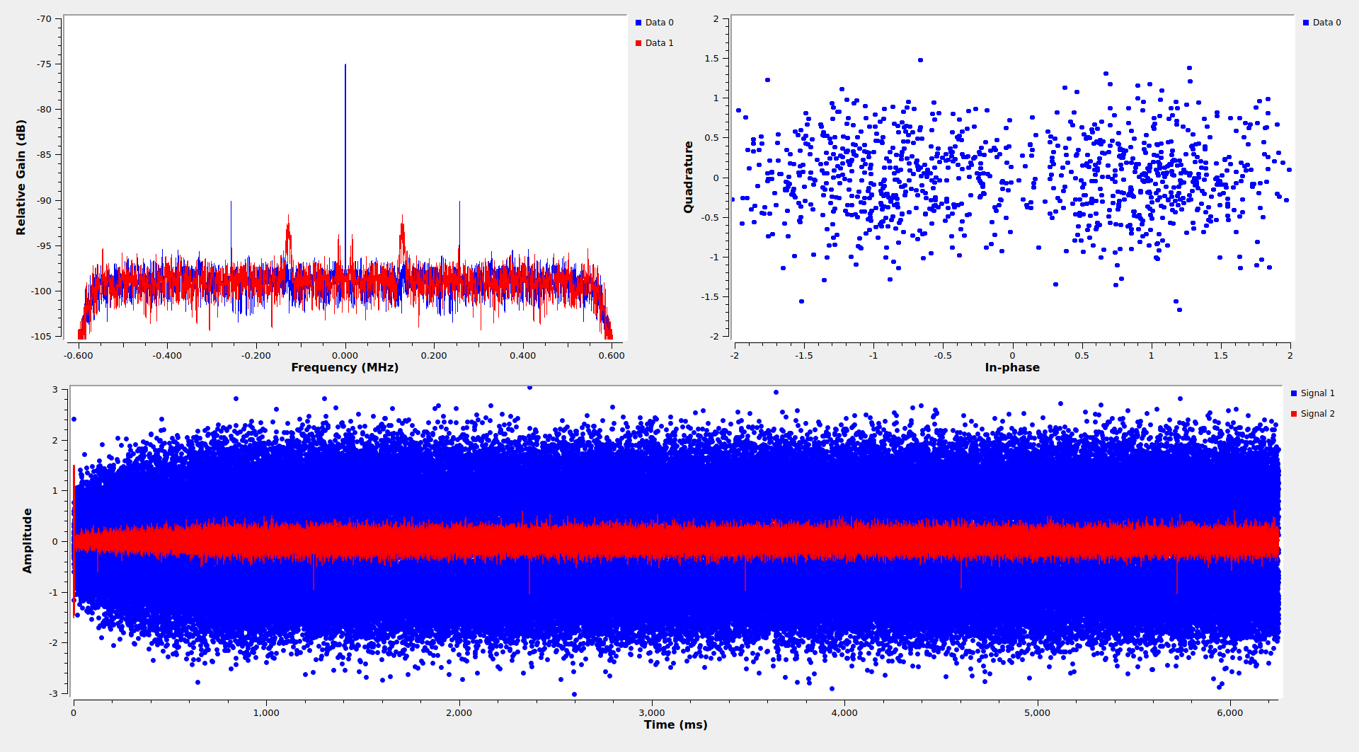
The figure below shows the GUI of the decoder flowgraph while running on the first recording. The top left plot shows the spectrum of the output of the PLL. We can see that the PLL has locked to the residual carrier correctly because the residual carrier appears only in the I component, and the data modulation in the Q component. The top right plot is a constellation plot of the telemetry modulation. The bottom plot shows the telemetry symbols in the time domain and their correlation with the 64-bit ASM used for r=1/2 Turbo codewords.
AOS frames
Hakuto-R M1 transmits CCSDS AOS Space Data Link frames, using spacecraft ID 0x38. This ID is assigned to HAKUTO-R-L1 in the SANA registry for the return link. The forward link has the spacecraft ID 0x184 assigned. We have been seeing this trend of using different spacecraft IDs for the forward and return links in the cubesats from the Artemis I mission.
Only virtual channel 2 is in use in the two recordings. There are no idle frames. The frames have a Frame Error Control Field (CRC-16), as recommended for Turbo coded data. This CRC is checked in the GNU Radio flowgraph. There is no Operational Control Field or AOS Insert Zone. In both recordings the SNR is good enough to decode without any lost frames.
Virtual channel 2 carries CCSDS Space Packets using M_PDU. The APIDs in use in the two recordings differ somewhat, but there are the following general aspects that apply to both. Idle packets in APID 2047 are used to fill up the packet data zone and complete an AOS frame when there is no more data to send. They have variable length (as required), no secondary header, and their data zone is filled with 0xdc bytes. This is characteristic of the IRIS v2 transponder, together with the use of virtual channel 2 for real time telemetry. We have seen this already in LunaH-Map and ArgoMoon, so it seems that Hakuto-R M1 also uses an IRIS v2.
The rest of the packets have a fixed length, which depends on the APID, and they have the secondary header flag enabled. There are a few packets with data length value of 61. In the first recording these appear in APIDs 136 and 264 (2 packets in each APID, which seem to have the same contents), and in the second recording they appear in APID 392 (3 packets). The majority of the packets are much larger. They belong to APID 1855 (with a data length of 874) in the first recording and to APID 1852 (with a data length of 779) in the second recording.
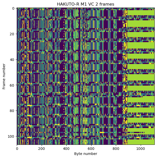
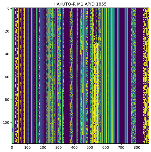
The figure below shows a raster map of the AOS frames in the first recording. The idle Space Packets can be identified by their characteristic yellowish green colour. We see that most frames carry a packet from APID 1855, which occupies a good part of the frame, followed by an idle packet that completes the frame. Sometimes this pattern breaks up, as two APID 1855, or packets from other APID, get sent in a row.
Here is a raster plot of the payload of the APID 1855 packets, taken from the first recording. There are more detailed plots, over each block of 128 bytes, in the Jupyter notebook. APID 1855 and 1852 are very similar in structure. Comparing them, the only major differences are that APID 1855 has some data in bytes 320-332, while APID 1852 has zeros in this section (this may be caused by a subsystem or instrument being disabled during the second recording), and that APID 1855 has some extra data at the end, owing to its larger size. The rest of the fields seem to be in the same positions and use the same format.
APIDs 1855 and 1852 seem to contain real time telemetry, and they occupy most of the telemetry link capacity. I have tried to reverse engineer the data they contain and have managed to make good sense of the ADCS data. There are many fields that are in float32 format, which makes this task slightly easier.
ADCS telemetry
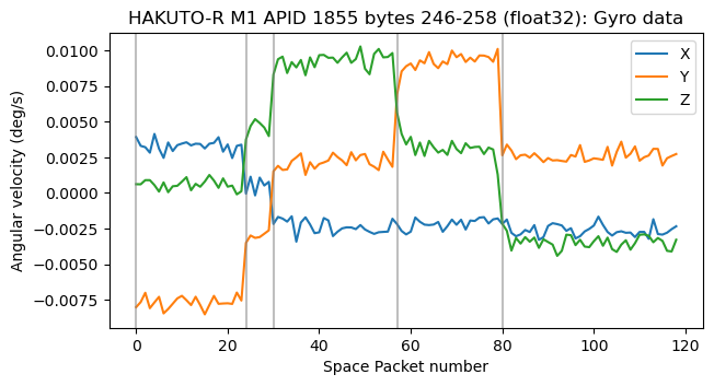
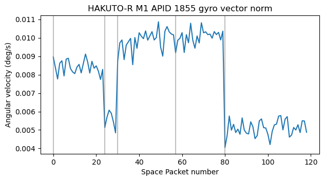
The figure below shows a plot of three float32 fields in the APID 1855 packets from the first recording. As we will find out, they correspond to gyroscope data, and their units are most likely deg/s. There are 5 distinct regions in the plot. The data is almost constant in each region, with jumps between the regions. This probably corresponds to small torques from the actuators changing the rotation (note that the rotation rate is always quite small).
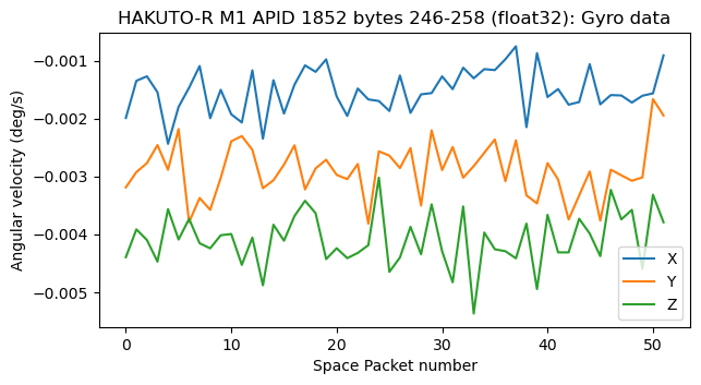
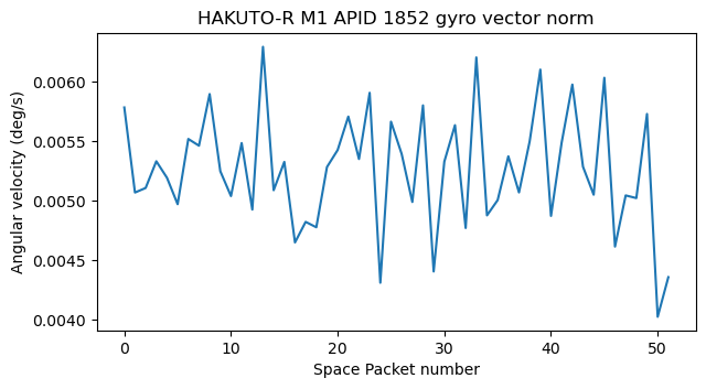
In the second recording we have constant data for the gyroscope channels. The values are also small.
The next four bytes in APID 1855 are shown below. They are unit quaternions describing the attitude of the satellite as a body frame to inertial frame rotation. The format is scalar last (the last component is the real part of the quaternion). We can check that the norm of the vector formed by these four numbers is one (except for rounding errors in the float32 format). Any time that the norm of four consecutive numbers is one (or another constant, which happens when integer instead of floating point format is used), it is very likely that they are attitude quaternions.
When looking at the telemetry of LunaH-Map, I also found some attitude quaternions, but there I wasn’t sure of whether they were in scalar last or scalar first format. Here, the presence of angular velocity data from the gyroscopes enables us to determine the format of the attitude quaternions, and to establish that the data shown above does indeed correspond to the gyroscopes.
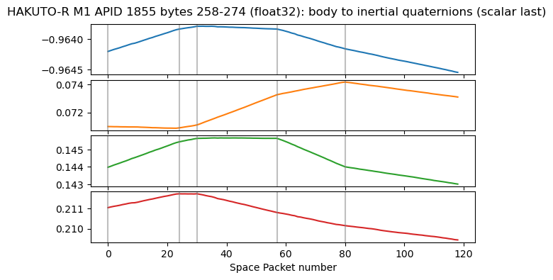
We can see that the quaternions change roughly in a linear way, with a different slope in each region. Their change throughout the recording is relatively small.
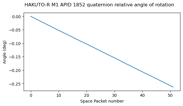
The corresponding data from APID 1852 is shown next. Here we only have a single slope in the data, which makes sense because the gyroscope values were constant. The values of the quaternions are similar to those in the first recording, so we see that the attitude of the spacecraft hasn’t changed much.
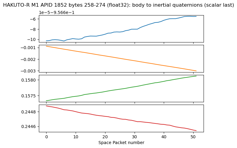
As usual, if \(q(t)\) denotes the attitude quaternions representing the body to inertial rotation, then \(q(t)^{-1}q(t_0)\) represents the relative rotation between time \(t_0\) and time \(t\), expressed in the body frame. The axis of this rotation, as well as its angular rate should match the gyroscope data (which is always expressed in the body frame, because the gyroscopes are attached to the spacecraft body). This check also verifies that the quaternions describe body to inertial rotations, rather than inertial to body rotations.
I haven’t tried to check what is the inertial frame used by the quaternions. This is not easy without some knowledge of the attitude of the satellite with respect to an external object (for example, knowing that the solar panels are pointed directly to the Sun would help a lot). However, it is quite likely that the inertial frame is ICRF or a similar system, such as J2000.
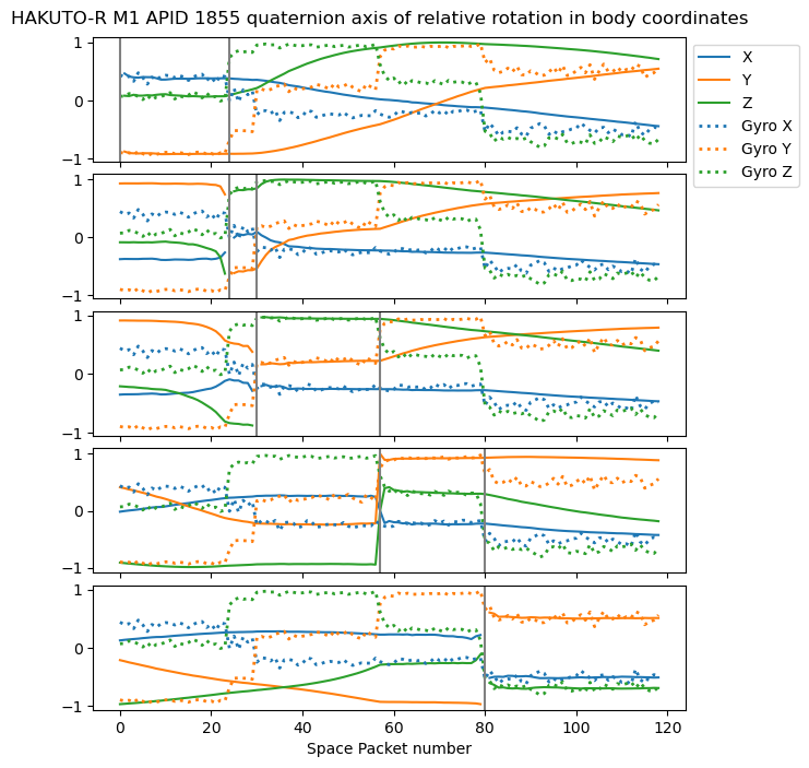
We can compute the rotation axis of \(q(t)^{-1}q(t_0)\) by normalizing the vector formed by the \(i, j, k\) components. We can compare this axis to the rotation axis described by the gyroscopes, which is the obtained by normalizing the gyroscope data vector. Since the first recording has a sequence of five different rotations, we do this procedure for each of the five rotations, taking \(t_0\) as the beginning of the time interval corresponding to each rotation. The results are show below. We can see a very good match between the rotation axes of the quaternions and the gyroscopes.
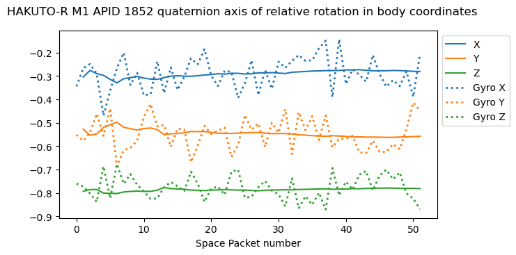
In the second recording we only have a single rotation. There is also good match between the gyroscopes and quaternions.
The next step amounts to checking that the rotation rate described by the quaternions matches the gyroscopes. So far, we have been able to work without a notion of the time variable (note that all the plots use “Space Packet number” as the x-axis). However, to relate the rate of rotation of the quaternions with the gyroscopes, we need to know the timestamps of the data, because we need to take derivatives or integrals with respect to time.
Unfortunately, I haven’t been able to find timestamps on the packets. The Space Packets have a secondary header, which is where the timestamp is usually located. But the data at the beginning of the packet doesn’t look like a timestamp. The next best thing that we can do is to timestamp the AOS frames, assuming that they get transmitted at the nominal baudrate, and then timestamp the Space Packets using the timestamp of the AOS frame that carries their first byte. We know that it takes 1.1195 seconds to send an r=1/2 Turbo coded 1115 byte AOS frame at 16 kbaud, and this is enough to give a relative timestamp to each frame.
In the first recording, usually there is a Space Packet from APID 1855 in each AOS frame, but sometimes there are two APID 1855 packets in a frame (well, a full packet, plus the beginning of another). We can compute the average rate at which APID 1855 packets get sent over the recording, obtaining 1.005 seconds . This comes suspiciously close to one second, so my interpretation is that the APID 1855 packets are generated at a rate of one packet per second. In the second recording, a similar thing happens with APID 1852. On average, there is one APID 1852 packet every 1.010 seconds. This agrees with the idea that these packets are generated at a rate of one per second. With this knowledge, we can now compare the rotation rates of the quaternions and gyroscopes.
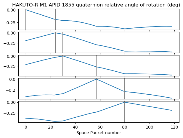
We can find the angle of the rotation \(h(t) = q(t)^{-1}q(t_0)\) as indicated here. For the first recording, we do this taking \(t_0\) at the beginning of each of the time intervals that correspond to different rotations. We find that in each time interval the angle changes linearly, consistently with a constant angular velocity.
In the second recording we also see a linear change of the angle of rotation.
We can obtain the rotation rate by taking the norm of the vector formed by the gyroscopes. We see that in the first recording the rate is constant in each of the intervals corresponding to different rotations, while in the second recording, the rate is constant throughout the recording.
So far I have been claiming that the units for the gyroscope data are deg/s, but I haven’t given any evidence for this. Now we can compare the rate of rotation according to the gyroscopes (averaging for each rotation), and the rate of rotation according to the quaternions, obtained by dividing the difference in angle over the time length for each of the intervals corresponding to different rotations.
Since the rotation rate according to the gyroscopes and to the quaternions should be equal, we can find the scale factor of the gyroscopes, or in other words, their units. In all the cases, the scale factor is very close to -1 deg/s, so besides a sign convention, this gives good support for the fact that the gyroscope data uses units of deg/s (which is a rather natural choice, moreover).
So far we have seen how having the gyroscope data together with the quaternion data is very helpful when reverse engineering the ADCS data. The gyroscopes constrain the format of the quaternions (scalar last vs. scalar first, and body to inertial versus interial to body), while the quaternions (which are unit-less) serve to find the units of the gyroscopes. Let us continue looking at the rest of the ADCS telemetry.
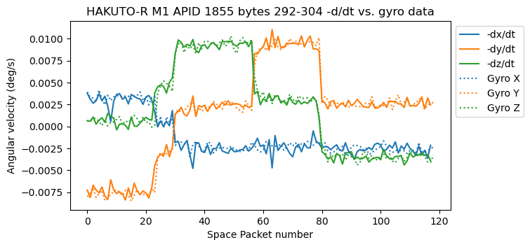
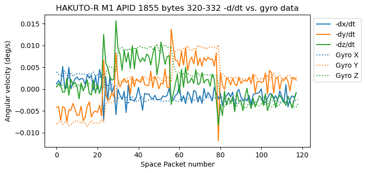
In bytes 292-304 and 320-332 of APID 1855 we have float32 triplets which look qualitatively similar. The derivative of the first of these is very close to the gyroscope data (with a change of sign). The derivative of the second is not so close to the gyroscope data (and is also much noisier), but still follows the same general trend. This gives good evidence that these data represent angular quantities in units of deg. I think that perhaps they represent the angular error, with respect to the desired attitude, because the values are small and seem to oscillate around zero.
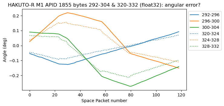
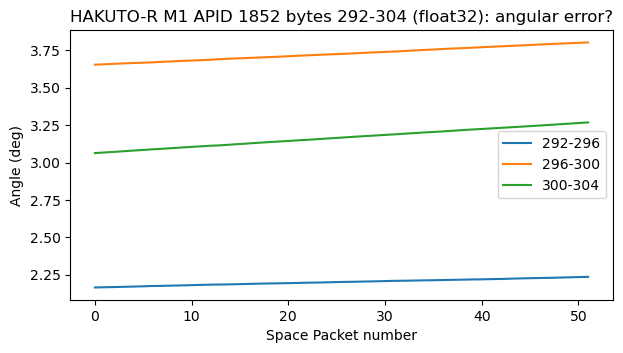
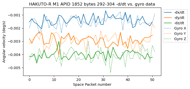
In the second recording, we only have data like this in bytes 292-304 of APID 1852. Bytes 320-332 in this APID only contain zeros. There is also good agreement between the derivative of this data and the gyroscope data. However, the values are now around 3 deg instead of around zero. This makes me wonder if they really represent angular error.
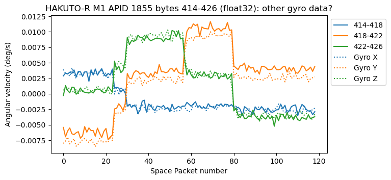
In bytes 414-426 of APID 1855 we have what seems to be data from a different set of gyroscopes. Perhaps a redundant set of gyroscopes using a different technology, and hence having different biases and accuracy. The plot below shows the comparison between this data and the gyroscope data in bytes 246-256. Note that there is a bias of ~0.002 deg/s in the Y component.
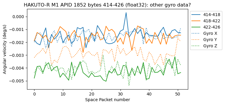
APID 1852 has the same kind of data in the same location. We can see the same bias in the Y component.
Finally, bytes 474-486 contain exactly the same gyroscope data as bytes 246-256, but with the opposite sign. This happens both in APID 1855 and APID 1852.
Other telemetry data
Here is some other telemetry data that has caught my eye, though I don’t have a good explanation for what it represents.
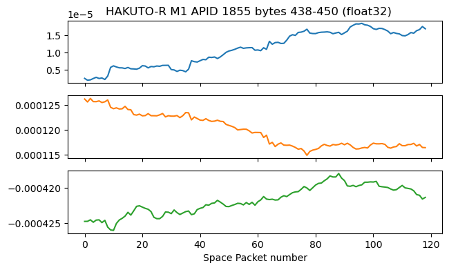
Bytes 438-450 of APID 1855 contain three float32 values.
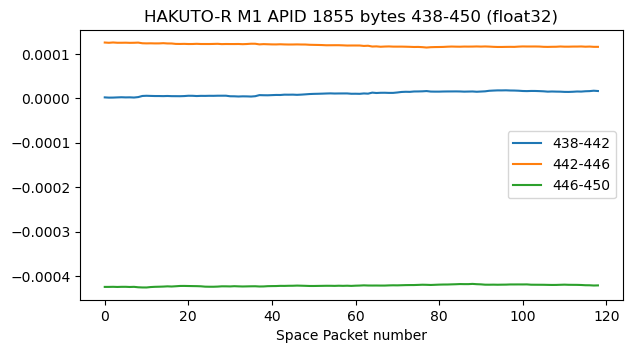
They change slowly, and in a noisy way. This is best seen when plotting each of the three values separately, as done below. They could be related to the ADCS, but I don’t know how to interpret them. The corresponding bytes in the APID 1852 in the second recording have a similar behaviour.
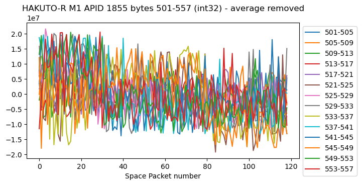
In bytes 501-557 we have 14 channels of what seems to be int32 data. These have somewhat noisy, almost constant values. Some values are around zero (and change sign, giving evidence for signed rather than unsigned data), while others are away from zero.
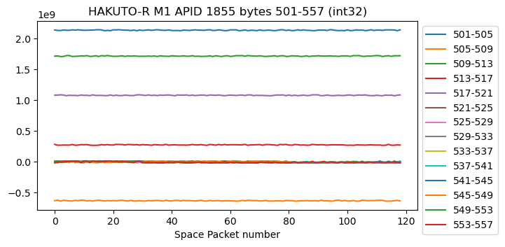
If we plot each channel minus its average, we can see the noise better. It also seems that some channels have some slope or other kind of slow variation. The data of these 14 channels in APID 1852 looks very similar.
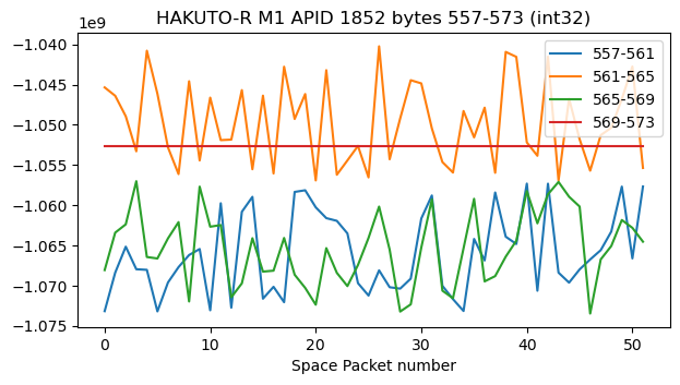
The next four channels also seem to be int32, but they look a bit strange because they change sign sometimes, producing huge jumps.
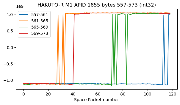
The corresponding data in APID 1852 in the second recording looks similar, but there are no sign changes and the fourth channel has a constant value.
Code and data
The GNU Radio decoder flowgraph and Jupyter notebooks used in this post can be found in this repository, together with the data files containing the AOS frames output by the decoder.
Thank you for such a thorough examination of this topic!
Google is failing me because there is so much focus on the math… in the context of bodies in space, would you mind terribly explaining in practical terms what “inertial frame rotation” is?
If I understand correctly, these quaternion values quantify the spacecraft’s deviation from a “perfect” line of flight, but I’ve not been able to fully understand (in a visual sense – not the math) what that “inertial frame rotation” point of reference exactly is.
Thanks as always.
Hi Scott,
An inertial frame is one that doesn’t accelerate or rotate. For instance, we often use the ICRF frame, which is defined by having Z point to the north pole, along the Earth’s rotation axis, X point in the direction of the point of Aries, along the intersection of the ecliptic and the equator, and Y completing the right-handed system.
Attitude quaternions describe de orientation (i.e., rotation) of the spacecraft in space. They don’t describe position, and they don’t describe deviation from intended trajectory or state. They describe the absolute orientation. It is common to describe this orientation by giving the rotation that would transform the spacecraft body frame into a given inertial frame, such as ICRF. The spacecraft body frame is defined differently for each spacecraft, but usually its definition involves important parts of the spacecraft such as solar panels or engines (for instance, see how it is defined for Tianwen-1 here).
To give an analogy, think about heading, pitch and roll for an airplane.