The QO-100 WB transponder is an S-band to X-band amateur radio transponder on the Es’hail 2 GEO satellite. It has about 9 MHz of bandwidth and is routinely used for transmitting DVB-S2 signals, though other uses are possible. In the lowermost part of the transponder, there is a 1.5 Msym QPSK 4/5 DVB-S2 beacon that is transmitted continuously from a groundstation in Qatar. The remaining bandwidth is free to be used by all amateurs in a “use whatever bandwidth is free and don’t interfere others” basis (there is a channelized bandplan to put some order).
From the communications theory perspective, one of the fundamental aspects of a transponder like this is how much output power is available. This sets the downlink SNR and determines whether the transponder is in the power-constrained regime or in the bandwidth-constrained regime. It indicates the optimal spectral efficiency (bits per second per Hz), which helps choose appropriate modulation and FEC parameters.
However, some of the values required to do these calculations are not publicly available. I hear that the typical values which would appear in a link budget (maximum TWTA output power, output power back-off, antenna gain, etc.) are under NDA from MELCO, who built the satellite and transponders.
I have been monitoring the WB transponder and recording waterfall data of the downlink with my groundstation for three weeks already. With this data we can obtain a good understanding of the transponder behaviour. For example, we can measure the input power to output power transfer function, taking advantage of the fact that different stations with different powers appear and disappear, which effectively sweeps the transponder input power (though in a rather chaotic and uncontrollable manner). In this post I share the methods I have used to study this data and my findings.
Assumptions
The main idea behind this post is that if we record waterfall data of the downlink, we are able to measure the relative power of the different signals in the transponder, as well as our receiver’s noise floor. If we do some reasonable assumptions, this allows us to estimate other quantities, which are in principle not directly measureable. These assumptions are the following:
- The transponder characteristics, such as its input to output power transfer function and its passband shape are constant over time.
- The effective G/T of my groundstation is constant over time. By effective G/T I mean the one which considers the antenna gain in the direction of the satellite. This assumption is not completely true because the effective gain can change slightly as the satellite moves around its GEO slot, and because the receiver system noise temperature can depend on the temperature of the LNB and other factors. This assumption allows us to relate our measurements to the received signal flux after a suitable calibration of the receiver gain by using the receiver noise floor as reference.
- The satellite antenna gain in the direction of my groundstation and the propagation losses are constant over time. Again, this is not completely true because the satellite might move somewhat and atmospheric losses depend on the weather. This assumption allows us to relate the received signal flux with the power transmitted by the satellite.
- The beacon signal power received by the satellite is constant. Note that this assumption involves a constant transmit power for the beacon as well as constant antenna gains in the groundstation and satellite, as well as constant propagation losses. This assumption will allow us to relate the power we observe at the output of the transponder with the power of signals at the input of the transponder. This is critical for this study, because we do not know the uplink powers of the signals that we see in the transponder. We will compare them to the beacon in order to establish a reference for transponder input powers.
Calibration
The first calibration that is applied to the recorded waterfall data is the bandpass calibration obtained in the previous post. This flattens the shape of the Pluto SDR passband. Then a scale factor is determined by hand and applied to make the receiver noise floor power in each FFT bin close to one (or 0 dB). This scales the waterfall data so that it measures power spectral density with respect to N0, the receiver noise in 1 Hz.
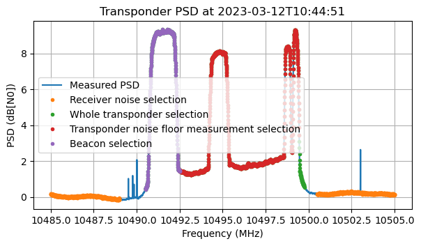
The figure below shows the power spectral density at the beginning of the recording. The following measurement areas are marked:
- Receiver noise: below 10489 and above 10500.5 MHz, avoiding a spur at 10503.02 MHz.
- Whole transponder: from 10490.5 to 10499.75 MHz.
- Transponder noise floor: from 10492.5 to 10499.45 MHz. (This can be occupied by stations, which we will detect and select out).
- Beacon: from 10490.5 to 10492.5 MHz.
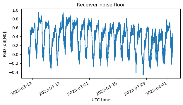
As I showed in the previous post, the gain of the receiver depends on several factors, including the temperature of the LNB. This makes it necessary to calibrate out the receiver gain. To do this, we use the assumption that the receiver G/T is constant. For each timestamp, we measure the average receiver noise floor using the area marked above and then divide the data by this value.
This figure shows the average power of the receiver noise floor versus time. It follows a daily pattern (higher gain at night, when the LNB is cooler), with an amplitude of around 0.8 dB.
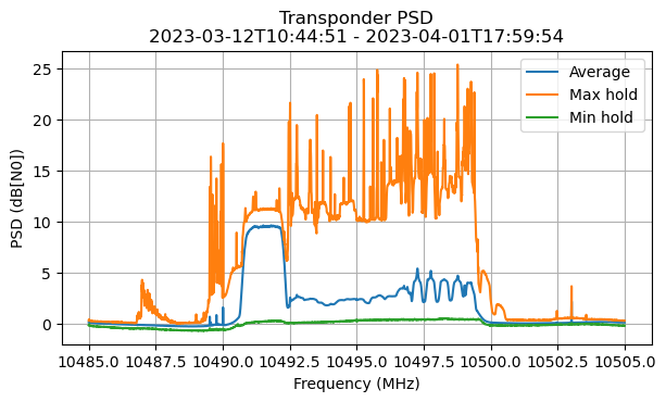
Here is the transponder PSD average, max hold and min hold over the whole duration of the waterfall data (about 3 weeks). This plot looks somewhat similar to the one I showed in the previous post, which only used one week of data.
The min hold and max hold show events which are worthy of further study, such as rather large signals in the transponder, and IMD skirts visible in the max hold, as well as occasions when the transponder noise floor and beacon are very depressed in the min hold, perhaps due to a very large signal present somewhere. However, this will be the topic of a future blog post.
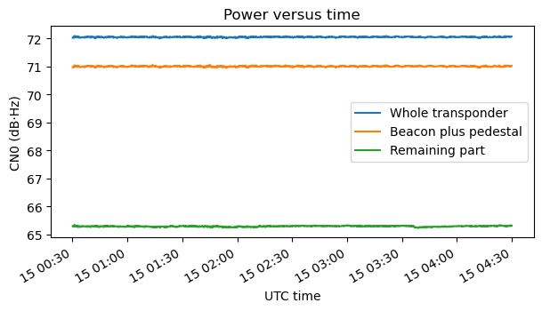
The next figure shows the powers of three regions of the transponder during the first three hours of data: the whole transponder; the beacon “plus pedestal”, which is the 2 MHz in which the beacon lives, including the transponder noise floor “pedestal” in this 2 MHz; and the “remaining part” of the transponder, which is actually the transponder noise floor measurement area (this includes both the transponder noise floor and any stations that are transmitting in this area). The power is measured with respect to the receiver noise floor in 1 Hz, so it is shown as CN0 in dB·Hz. The contribution of the receiver noise floor has already been subtracted from all these measurements.
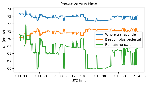
This data corresponds to a Sunday morning, so several stations are active and we can see the power of the remaining part jumping up and down as different stations start and stop transmitting. We see that the power of the beacon changes by up to 2 dB. When there is more power in the remaining part of the transponder, some power is robbed from the beacon. We will look at this in more detail later.
The next step in calibration is to measure the shape of the transponder noise floor. I will explain later why we need this. It is clear from some of the plots that the noise floor is not flat. It is somewhat sloped, increasing in power as frequency increases. This can also be seen in the Goonhilly WebSDR, so it is not an effect of my receiver.
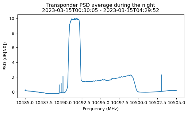
To perform this measurement, I have selected a time interval during the night, when no stations other than the beacon are active, and the power levels are very stable. On the night of March 15 there are 4 hours of data that can be used.
This shows the average power spectral density during this 4 hour period. As expected, we can see that there are no stations other than the beacon.
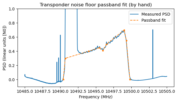
In have fitted a piecewise linear function by hand to the power spectral density of the transponder noise floor in linear units.
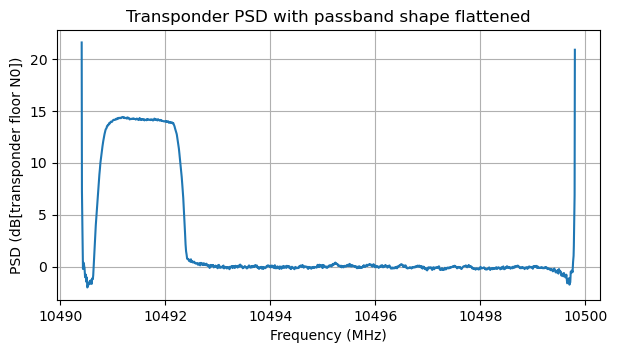
We can use the fitted passband shape to flatten out the transponder noise floor. The results applied to the PSD average over the night of March 15 (minus the contribution of receiver noise floor) are shown here. We can see that the passband shape makes a poor job at characterizing the transponder skirts, but the passband is now quite flat.
In this flattened passband we are going to detect using a threshold the frequency bins in which signals are present in the transponder noise floor measurement area. These bins will be ignored, and the transponder noise floor level will be measured as the average of the (flattened) power in the remaining bins. The goal of this is to obtain a measurement of how much transponder output power is spent in the transponder noise floor.
The reason of flattening the passband before doing this measurement is that otherwise we would obtain biased results depending on where in the passband the stations are transmitting. For instance, if stations are active in the higher frequencies, then our average over the unused frequencies would be an underestimate, since we would be ignoring the part of the transponder in which the noise floor is higher.
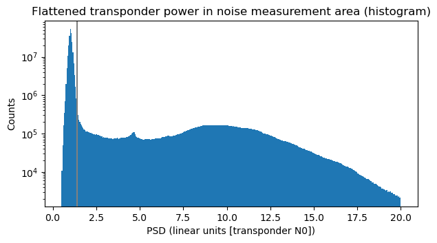
To obtain the threshold that determines whether an FFT bin is occupied by a transmission, we plot the histogram of the FFT bins of the flattened transponder power in the noise measurement area over all the time duration of the data. In the histogram we can clearly see the region corresponding to FFT bins which do not carry any signals as a narrow and tall hump on the left, and the region corresponding to FFT bins carrying signals as a wide plateau. This helps us select a threshold, shown as a vertical grey line.
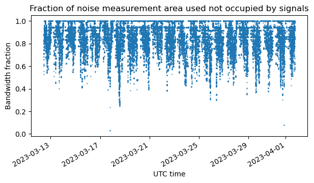
The next figure shows, for each timestamp, the fraction of the bandwidth of the noise measurement area that is not occupied by signals, according to the threshold we have defined. This is an indicative of the transponder activity. We can see periods when this region of the transponder is completely free. This tends to happen during the night, for instance. We can also make out some horizontal lines at bandwidth fractions smaller than one. These appear because typically signals have a discrete set of bandwidths: 125 ksyms, 250 ksysm, 333 ksysm, 500 ksyms and 1 Msym.
The transponder noise floor level is now measured, for each timestamp, as the average of the FFT bins not occupied by signals in the flattened noise selection area. The next figure shows the transponder noise floor level over time in dB units relative to the night of March 15 (which we have used as reference to measure the shape of the noise floor).
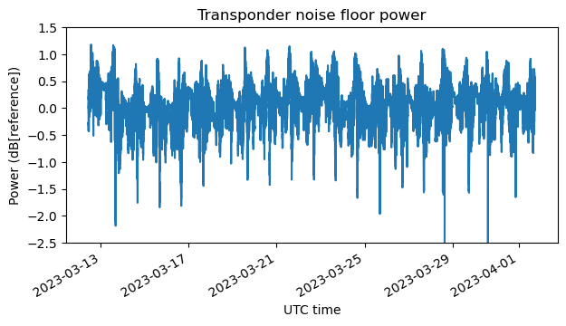
We can see relatively fast variations. These are caused by stations appearing and disappearing, which as we will see below changes the operating point of the transponder (with respect to compression) and makes the noise floor power change (in the same change that the beacon power changes, as we saw above). There are also much slower changes, with a timescale of a few days. I don’t know what causes this. Maybe the G/T of my antenna is not constant, or the transponder parameters (output power, etc.) change somewhat. This slow variation indicates that our initial assumptions are not completely true, but the changes are at most 1 dB.
Measurement of the beacon power
Now that we have measured the shape of the transponder noise floor and how the transponder noise floor level changes versus time, we can measure the power of the DVB-S2 beacon. Above we were considering the power of the beacon “plus its noise pedestal”. We can compute the power of the noise pedestal as the integral of the transponder noise shape over the beacon bandwidth multiplied by the transponder noise level. Then we can subtract the power of the noise pedestal to obtain only the power that is due to the beacon.
The plot below corresponds to the first three hours of data. It shows the power of the whole transponder, the power of the beacon (this time without its noise pedestal), the power of the remaining part of the transponder (including the transponder noise floor on this area), and the power of the transponder noise floor measured over the whole transponder.
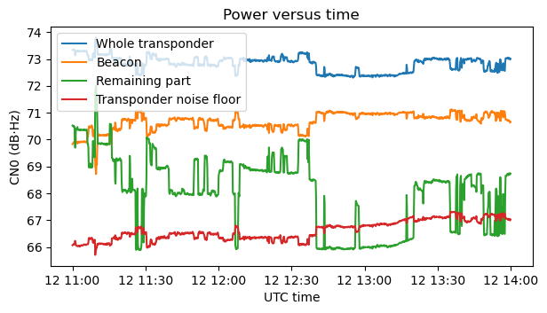
We can now see that as stations start and stop transmitting, the beacon and the transponder noise floor change by almost the same amount. This is best seen in the next figure, which shows only these two traces with their averages (in dB) subtracted for easier comparison.
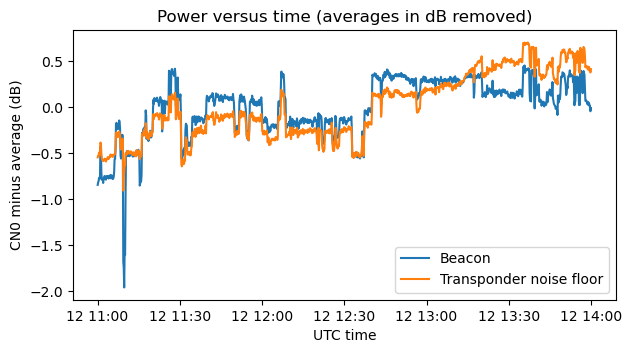
The reason for these changes is that, as we will see next, the transponder is operating somewhat in compression. The beacon and the transponder noise floor (understood as the equivalent power at the transponder input) have constant power at the input of the transponder. As more input power appears in the form of additional stations in the “remaining part” of the transponder, the transponder is driven more and more into compression. Effectively this reduces the gain of the transponder, so the additional stations rob the beacon and transponder noise floor of some of their downlink power.
In the plot above we can see that although the beacon and transponder noise floor change in a very similar way, they are not quite the same. The transponder noise floor is increasing a little over this 4 hour period. Perhaps this is due to the fact that the transponder input noise is changing over time (it could also be a change in noise figure or other parameters). I heard that most of the contribution to the uplink antenna temperature is caused by the thermal noise of Earth, instead of the millions of unlicensed devices running in the 2.4 GHz band. If so, perhaps using this kind of measurements we could detect the change in average Earth temperature over the transponder footprint, which follows a day and night cycle. This is an interesting thought, but somewhat off-topic, and probably not trivial to carry out due to many nuisance factors, such as stations appearing and disappearing.
Transponder input to output power transfer function
We are now ready to measure the transponder input power to output power transfer function. The output power is something that we have measured directly. It is the data we have been plotting as “whole transponder” power. To compute the input power, we use our assumptions. These imply that the input power of the beacon into the transponder is constant. Therefore, the gain of the transponder is proportional to the output power of the beacon (which we have just measured above). Dividing the output power by the gain, we obtain the input power.
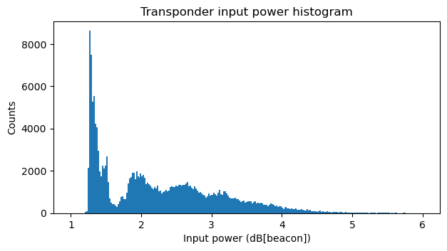
The figure below shows a plot of our input power and output power measurements in dB units, as well as a fit of a degree 2 polynomial to this data. The input power is measured in dB relative to the beacon input power. For instance, an input power of 3 dB would mean that the input noise and other signals have the same input power as the beacon. Note that the input power never gets below 1.25 dB or so because, in addition to the beacon, we always have the equivalent input noise for the transponder noise floor present at the transponder input. The output power is measured as CN0, relative to the receiver noise floor power in 1 Hz.
This plot shows that the transponder is operating in compression. If the transponder was in its linear region, then a change of 1 dB in input power would produce a change of 1 dB in output power. However, we see that over a range of 5 dB in input power the output power only changes by 1.5 dB or so.
Even with only the beacon present, the transponder is already in compression. From the polynomial fit (and also from some of the most extreme measurements), it appears that the maximum output power that the transponder can deliver is 73.5 dB·Hz. With only the beacon present the tranponder is already at 72.25 dB·Hz output power. This is pretty much 1 dB output power back off with the transponder “free” (besides the beacon, which is always present).
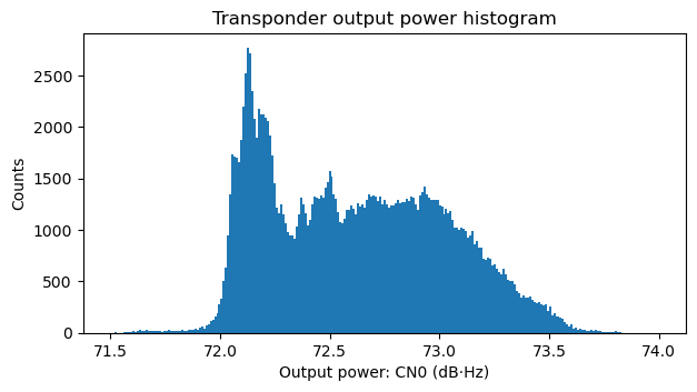
Even thought the density of the points in the plot above gives an indication of how frequently each of the input power and output power situations happen, it is interesting to look at histograms of the relevant quantities. These are shown below.
Transponder output power budget
We now study the transponder output power budget. To do this we need to fix an operating point. Looking at the transfer function plot above, it seems that the highest reasonable operating point that we can choose is 73 dB·Hz. This is about 0.5 dB output power back off. Above this level the transponder is really saturated and probably produces high levels of distortion. The operating point of 73 dB·Hz output power corresponds to an input power of 3 dB[beacon]. This gives a nice round number, because it means that at this operating point the beacon will occupy 50% of the power budget, with the remaining 50% to be divided between the transponder noise floor and other signals.
To determine the amount of output power that is spent by the transponder noise floor, we integrate the transponder noise floor shape over all the transponder bandwidth and average the measurement of the transponder noise level over all the time. This gives us an indication of the average power spent in transponder noise floor. We obtain 66.2 dB·Hz.
To be more precise, we would need to consider that the total input power of the transponder changes the output power allocated to the transponder noise floor, because the transponder gain changes. However, we have also seen that the transponder noise level changes because of other reasons (for instance, in the plot of the first three hours of data we can see the transponder noise changing by 1 dB, even if we correct for the jumps in power caused by stations appearing and disappearing). Therefore, it seems reasonable to take an average, knowing that it is perhaps accurate to 1 dB.
We can now give a transponder output budget for the case when the beacon is not present. This would correspond to the situation where the beacon is removed, and all the transponder power and bandwidth is available for use by other stations. It is a good exercise. Taking into account that 66.2 dB·Hz are spent by the transponder noise floor, this gives 72 dB·Hz of power available to signals.
The important question from a communications theory perspective is: if all these 72 dB·Hz of power were used by a single signal occupying the full 9 MHz of transponder bandwidth, what would its SNR be? Here I am using a single signal just for simplicity. If we divide the transponder bandwidth into several signals, this post shows that the maximum total channel capacity is achieved when power is allocated to each signal proportionally to its bandwidth, so that all of them have the same SNR (this situation is exactly what I had in mind when I wrote the post).
To answer this question, we need to take the receiver noise into account. In fact, most of the noise that we get in the receiver is receiver noise rather than transponder noise. Indeed, the receiver noise power over a 9 MHz bandwidth is 69.5 dB·Hz. This is the only point in this study in which the G/T of my station becomes relevant. A station with a different G/T will see all the figures I’m giving in dB·Hz scaled up or down accordingly, and so the final SNR will change.
Therefore, it is relevant to mention that my station has a 1.2 m offset dish, but the system noise temperature is not so good (it is around 250 to 330 K, according to some measurements I have done). In this aspect, my station is probably better than the average QO-100 groundstation, due to the larger dish, but probably not by much, due to the relatively large noise temperature. For relative comparisons with other stations, we can take the G/T of my station as 15.5 dB/K. For more information, see this post.
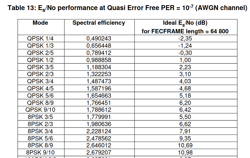
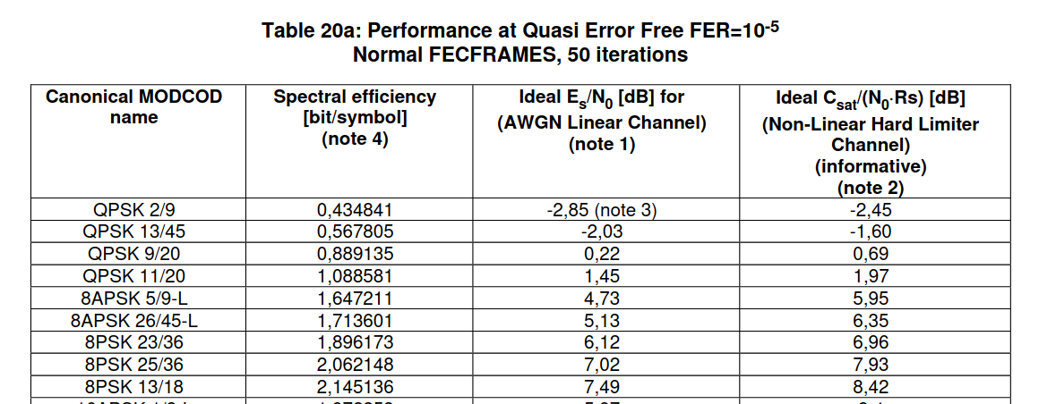
So, assuming that my station is the receiver, this 72 dB·Hz signal occupying the full transponder bandwidth will have an SNR of 0.7 dB. According to the Shannon-Hartley theorem, the maximum spectral efficiency at this SNR is 1.12 bits per second per Hz. With a real world communications system we will achieve somewhat lower efficiency. It is interesting to look at the DVB-S2 error performance table to see the best DVB-S2 MODCOD that would work in these conditions. We have QPSK 2/5, which works at -0.3 dB Es/N0 and gives a spectral efficiency of 0.79 bits/symbol. Note that in doing this comparison I’m ignoring the RRC excess bandwidth, but it still gives a rough idea of what is possible to achieve with DVB-S2.
Now we will consider the more realistic output budget in which the DVB-S2 beacon is present. We will see how the SNR for the other stations changes given the fact that the DVB-S2 beacon occupies less than 2 MHz but spends 50% of the transponder output power budget.
First we determine the output of the beacon when the transponder is not used by other signals. To help us, we plot again the histogram of the beacon power (this time in linear units of power and with a logarithmic vertical scale). We see a small hump in the histogram that corresponds to this situation. We take the centre of this hump (marked as a grey vertical line) as the beacon output power. This gives 70.79 dB·Hz. A measurement of the average beacon power over the night of March 15 (when no other signals were present) gives 70.78 dB·Hz. This validates our measurement of the beacon power.
However, this is the beacon downlink power when the transponder is “free”. Since we have decided an operating point of 73 dB·Hz, the output power of the beacon will be somewhat less. We need to compute how much power is robbed from the beacon when we increase the operating point by adding other signals. The easy way to do this is to remember that, just by coincidence, with our choice of operating point the beacon spends 50% of the output power. Therefore, its power is 70 dB·Hz.
Another way to proceed is to calculate the gain reduction as the difference between the increase in output powers (from 72.1 dB·Hz to 73 dB·Hz) minus the increase in input powers (from 1.3 dB[beacon] to 3 dB[beacon]). This gives a gain reduction of 0.8 dB, so we again obtain a beacon output power of 70 dB·Hz by subtracting a 0.8 dB gain reduction from the 70.8 dB·Hz that we had determined for the case when the transponder is “free”.
Since the beacon spends 70 dB·Hz of output power, and we still assume that the transponder noise floor spends 66.2 dB·Hz of output power, we have 67.6 dB·Hz of output power for other signals. The SNR of these signals over the bandwidth of approximately 7 MHz that is available to them is around -2.70 or -2.77 dB depending on whether we consider the slope of the transponder noise floor shape or not (this detail doesn’t make a huge difference). The maximum spectral efficiency according to Shannon-Hartley for this SNR is 0.6 bits per second per Hz. Looking at the table above we see that DVB-S2 cannot even work at this SNR. This means that when the beacon is present, the remaining part of the transponder is completely in the power-constrained regime. It is not possible to make use of the 7 MHz of remaining bandwidth with DVB-S2 signals.
DVB-S2X includes an interesting QPSK 2/9 MODCOD that can work at -2.85 dB Es/N0. It is possible that with this MODCOD the 7 MHz bandwidth of the transponder could be used.
At the operational point of 73 dB·Hz, the DVB-S2 beacon has an Es/N0 of 7 dB. This means that it could use 8PSK 2/3 for a spectral efficiency of 1.98 bits/symbol. It is currently using QPSK 4/5, which gives a spectral efficiency of only 1.59 bits/symbol. Conversely, since QPSK 4/5 works down to 4.7 dB Es/N0, it would be possible to reduce the beacon power by up to 2.3 dB. This would free up a lot of output power budget for other signals. However, the rationale of having a relatively large link margin on the DVB-S2 beacon is so that even really small stations are able to receive it.
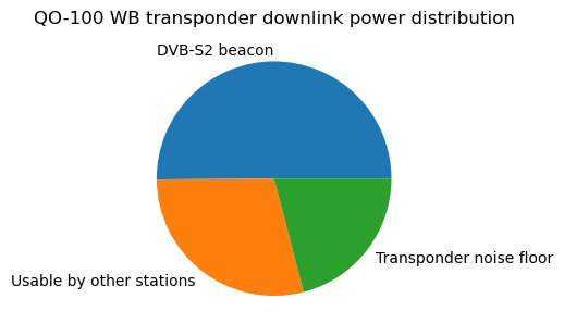
The transponder output power budget is best expressed as plots, which give an immediate visual impression of the situation. The following is the typical pie chart, which shows the output power distribution when the DVB-S2 beacon is present.
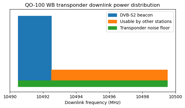
Another interesting way of plotting the powers of the different categories is as rectangles whose area is proportional to power and whose base is proportional to bandwidth. This means that the height of the rectangles is proportional to the power spectral density. This kind of plot allows visual comparison of power spectral densities in linear units. In this sense it is much better than the typical spectrum plot, in which power spectral densities appear in dB units, which can be visually misleading.
Here is this kind of plot. It makes it immediately clear that the DVB-S2 beacon can afford much higher power spectral density than the other stations. It also helps compare the power spectral density of these signals with that of the transponder noise floor. I think this plot is somewhat complementary to the pie chart, because it is not so easy to compare the areas of rectangles with very different aspect ratios.
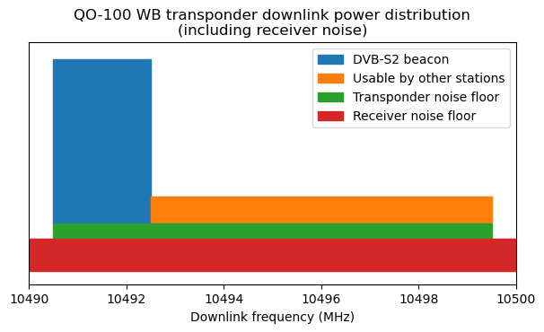
This plot doesn’t tell the whole story, because besides the transponder noise floor, there is the receiver noise. As we have calculated above, this is typically higher than the transponder noise, and sets the receive SNR. The next plot includes the receiver noise floor for my station. Its height is proportional to its power spectral density. This allows a quick visualization of the SNR of signals by comparing their height with the sum of the heights of the transponder and receiver noise floor.
Conclusions
In this post we have seen how using recorded waterfall data from the QO-100 WB transponder downlink we can estimate the transponder input power to output power transfer function, decide an operating point for the transponder, and compute an output power budget. The exact quantitative results should be taken with some (small) uncertainties, due to the indirect measurements and calibrations required, but I’m confident that the main results are accurate.
My main goal with this post is to understand better how the transponder power is distributed, and to invite reflection on how we could use the transponder resources (power and bandwidth) more efficiently. I don’t want to push people into changing their operating practices by any means. A change in operating practice should only follow careful study and decision making by AMSAT-DL, BATC and the wider community, and be reflected in a change of the operating guidelines.
I also want to show how some concepts in communications theory, such as channel capacity and spectral efficiency can be used as engineering guidelines in optimizing the use that we make of the transponder.
The results from this study show that some of the ways in which we use the transponder go against what the communications theory says, and that there is room for improvement. I think one important aspect of this is that bandplanning and operating guidelines for the transponder have traditionally focused mainly on occupied bandwidth, and not on power. This makes sense, because it is easier to regulate and measure bandwidth than power. However, this post shows that, specially when we consider that the DVB-S2 beacon is present, the transponder is much more power limited than bandwidth limited. Therefore, focusing on power usage should be more important than bandwidth.
I must say that I am somewhat surprised by the results of the study, specially the fact that the transponder is already in compression when only the beacon is active. However, I don’t see any large errors in my calculations and methods, and in hindsight the results seem to agree with what we observe qualitatively on the transponder. I guess that studies with somewhat surprising or not obvious outcomes are the most worthy to make.
Two of the main results are related: the transponder is close to saturation, even when it is “free” (only occupied by the beacon), and the beacon takes up 50% of the transponder power. I have mentioned why it can be reasonable that the beacon is designed with a relatively high link budget. Additionally, the beacon can be useful for outreach and gives well deserved publicity to QARS and Es’hailSat. On the other hand, it has been transmitting the same content for more than 4 years already. Therefore, it is natural to ask whether the beacon deserves to take up 50% of the transponder power.
In March 2020 the beacon configuration was changed from the initial 2 Msym QPSK 3/4 to the current 1.5 Msys QPSK 4/5. I believe that the beacon power was kept the same or didn’t change much. The intention of the change was to make more bandwidth available to other stations. This seemed to make sense (indeed it seemed very reasonable to me before I made this study), but now that we find that it isn’t really possible to use the 7 MHz of spectrum that are available to the other stations, we see that perhaps the reduction in bandwidth of the beacon perhaps didn’t accomplish what was intended.
A related matter regards the power spectral density of the other stations. The current operating guidelines say the following regarding transmission power.
All uplink transmissions should use the minimum power possible. QPSK transmissions should have a downlink signal with at least 1 dB lower power density than the Beacon – the web-based spectrum monitor enables users to set their uplink power to achieve this. Transmissions with symbol rates of less than 333 kS using 8PSK, 16 APSK or 32 APSK should use the minimum power density required to achieve successful reception.
Note that here “1 dB lower” is understood in terms of power spectral density or energy per symbol, not in terms of total power (which would naturally scale with bandwidth). Although I haven’t checked how frequently people abide by this rule (the waterfall data I’ve collected enables us to study this), I would say that my impression is that in general people follow it (give or take 1 or 2 dB). The WebSDR helps by displaying the power spectral density in dBb (dB with respect to the beacon) and by showing an “over power” warning for stations with too high power spectral density.
It is convenient to comment that this “1 dB lower”, and other WebSDR-based measurements are usually interpreted in terms of (S+N)/N rather than S/N, since this is what a spectrum display shows. However, the distinction is not too important for my comment.
What happens with this recommendation is that effectively people adjust their transmissions to have slightly less power spectral density that the beacon. This is no good. As we saw above, the beacon has 7 dB Es/N0, but the 7 MHz area that is available to other stations cannot support anywhere near this power spectral density, given that it only has around 30% of the transponder output power budget. In this sense, the beacon has 66% more power available than all the other stations combined. If the other stations ran at the same power spectral density, they could only occupy about 1 MHz before exhausting all the transponder power.
Communications theory tells us that in a 7 MHz channel with -2.7 dB SNR (which is what the other stations have available), it is better (in terms of achieving more bits per second) to use lower coding rates and larger bandwidths. We have seen that none of the DVB-S2 modes can support -2.7 dB SNR, but there is QPSK 1/4. As long as the beacon is present with its current power and bandwidth, the remaining power and bandwidth would be more efficiently used if everyone running DVB-S2 used QPSK 1/4 (using accordingly higher symbol rates) with the minimum power required (-2.35 dB Es/N0 according to the documentation, plus some reasonable link margin).
I don’t have a good notion of the DVB-S2 MODCODs that are more frequently used in the WB transponder, but I have the impression that people typically use QPSK 3/4 and above. This is not a good way to make use of a channel with -2.7 dB SNR. In fact, coming back to the topic of too much focus on bandwidth usage, I think that at some point it was encouraged that stations used narrower bandwidths and higher order modulations to get the same data rate. This makes a lot of sense for experimentation purposes (after all, the WB transponder should also be a platform where people can experiment what happens with all the MODCODs in different situations, within reasonable constraints), but it goes in the opposite direction of optimizing the transponder power/frequency usage.
One of the reasons why I wanted to collect waterfall data was to compute some statistics about the transponder usage, and in particular find out how frequently the transponder is “full”, in the sense that it cannot really accept more users. I was intending to simply look at the bandwidth occupied by the stations. However, now I realize that I actually need to look at the transponder output power (or equivalently, the input power). I will never see stations using the full 7 MHz of bandwidth being used, because it is impossible to do so with DVB-S2, specially with QPSK 3/4 and above. At this point everyone would be fighting for power, with the transponder heavily saturated, and none of the signals would have enough downlink SNR. I think this situation is very rarely reached in practice because before this happens people realize that the transponder is too busy and that they cannot put out a decent downlink signal, so they quit and go do something else. In this sense the transponder usage is some sort of closed loop feedback system.
Looking at the histograms, we see that in a small number of occasions the transponder was running at a rather high input power between 4 and 5 dB[beacon]. According to the input to output power transfer curve, here the transponder is very saturated in comparison with the 3 dB[beacon] operating point I have proposed. Compared to the operating point, people need to increase their uplink power by 1 or 2 dB only to gain 0.25 or 0.5 dB of downlink power. Additionally, what happens is that the beacon doesn’t increase its uplink power. In this sense, running the transponder so close to saturation is a way of robbing some more beacon power in trying to support more users. The users do need more uplink power than normal, because now the transponder gain is reduced, so everyone is fighting for power. It would make sense to have less beacon power to begin with.
A final comment regards the power allocated to the transponder noise floor. Roughly speaking, the beacon gets 50% of the power, the other users get 30%, and the remaining 20% goes to the transponder noise floor. This is an undesirable consequence of having a sensitive transponder. The way to reduce the power allocated to the noise floor would be to reduce the transponder gain, so that uplink signals need to be stronger, and thus present a higher SNR at the transponder input, to achieve the same downlink power. This might seem a good way of extracting more power from the transponder to support additional users. However, I think this would go against everyone, since it requires an increase in uplink powers, leaving smaller stations out of the game.
Code
The calculations and plots shown in the post have been done in this Jupyter notebook. As I mentioned in the previous post, I haven’t published the waterfall data anywhere because this is a file that still keeps growing and is already 2.8GB. If anyone wants a copy of the file to do an independent analysis, just let me know and I’ll figure something out.
One comment