Last week I wrote a post with a study about the QO-100 WB transponder power budget. After writing this post, I have been talking with Dave Crump G8GKQ. He says that the main conclusions of my study don’t match well his practical experience using the transponder. In particular, he mentions that he has often seen that a relatively large number of stations, such as 8, can use the transponder at the same time. In this situation, they “rob” much more power from the beacon compared to what I stated in my post.
I have looked more carefully at my data, specially at situations in which the transponder is very busy, to understand better what happens. In this post I publish some corrections to my previous study. As we will see below, the main correction is that the operating point of 73 dB·Hz output power that I had chosen to compute the power budget is not very relevant. When the transponder is quite busy, the output power can go up to 73.8 dB·Hz. While a difference of 0.8 dB might not seem much, there is a huge difference in practice, because this drives the transponder more towards saturation, decreasing its gain and robbing more output power from the beacon to be used by other stations.
I want to thank Dave for an interesting discussion about all these topics.
Input power to output power transfer curve review
While reviewing my study, I have not found anything terribly wrong with the methods and calculations themselves (though I have found a way to improve the calculation of transponder noise power, with which I wasn’t too happy). It was the interpretation of results what was more problematic.
To begin, let us review my plot of the transponder input to output power function. Here we can see that the transponder is close to saturation, even when only the beacon is active (which corresponds to the leftmost part of the curve). The transponder maximum output power seems to be slightly below 74 dB·Hz.
Additionally, the histogram of output power shows that most of the time the transponder is below 73.5 dB·Hz output power.
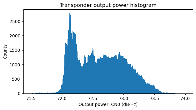
With this data in view, I had decided to run my output power budget analysis for an output power of 73 dB·Hz. I imagined that above this value there would be too much distortion on the transponder. Moreover, I had thought that a difference of a fraction of a dB, if we chose a higher output power, wouldn’t make much impact to the results. As we will see, this is wrong, because what fraction of the total output power is available for use by stations other than the beacon depends a lot on this. As the histogram shows that the events where the output power is around 73.8 dB·Hz happen very infrequently, I had decided to ignore these, thinking that they would perhaps correspond to brief moments in which a station mistakenly was transmitting too much power.
A case with a very busy transponder
After hearing Dave’s comments, I looked in my data for the events where the transponder output power was above 73.8 dB·Hz. This happens in several occasions over a 30 minute period on the evening of March 25 (a Saturday), and also in some occasions on the evening of March 31 (a Friday).
The following plot shows the transponder output power between 21:00 and 22:00 UTC on March 25. We can see that sometimes when there are many stations the output power goes above 73.8 dB·Hz, and even close to 73.9 dB·Hz.
Here is the waterfall corresponding to the same period. We can see that there are a lot of stations active, and the transponder bandwidth is almost full, taking into account guardbands between signals. We can see large changes in the power of the beacon (and also of other signals) as the number of active stations changes.
In this waterfall plot, there is some intermodulation distortion visible, as faint narrow signals around the three narrowband transmissions (in this sense, these transmissions almost play a similar role to a two-tone test). We will see more details about distortion later on, but I want to emphasize that the distortion is nowhere near the point where the transponder cannot be operated normally. The amount of distortion present in this situation seems perfectly tolerable. Therefore, rather than using 73 dB·Hz as the output power to work out a power budget, it seems much better to use 73.8 dB·Hz, which is representative of a situation where the transponder is very busy. I will work the details below.
I have selected one of the moments in the evening of March 25 in which the transponder output power was highest. The spectrum at this moment (a 10 second average, actually) is shown below. For comparison, I have also included the spectrum of a 15 minute average taken a couple hours later, when the only station active was the beacon. This helps compare the situations in which the transponder is very busy and “empty”. I have selected the closest moment in which the transponder is empty to try to eliminate any slow or long term biases in the measurement set up.
One of the shortcomings of my study is that it was difficult to verify the results independently. For instance, the input power to output power plot involved several calibrations and using 3 weeks worth of data. There is no way of independently obtaining this kind of plot without rewriting similar code from scratch and using all the data.
For this reason, I have decided to show here a spectrum measurement, with a fine grid with 0.2 dB spacing (it is possible to click on the plot to view it in full size). This makes it easy for anyone to review the main calculations and results using this spectrum and simple math that can be even carried out with pen and paper. Also, spectrum plots are reasonably easy to obtain with any other station.
A disadvantage of spectrum plots in a dB scale, such as the one above, is that they make it easy to compute (S+N)/N in dB units, simply by subtracting two values. However, this value then needs to be converted to S/N in dB units. This is done with the formula\[10\log_{10}\left(10^{x/10} – 1\right),\]where \(x\) is the (S+N)/N in dB units.
For this reason, I prefer to use a linear scale instead of dB. This allows to measure S/N in linear units by subtracting two values. If needed, we can convert the S/N to dB units with the formula\[10\log_{10} y,\] where \(y\) is the S/N in linear units. This is the same plot in linear units. Note that the three narrowband stations go off-chart. This is the disadvantage of a linear scale.
Here is another linear scale plot that shows the three narrowband stations.
In the plots above, we see that the transponder is used simultaneously by the beacon (1.5 Msym 4/5 QPSK), two 1 Msym stations, a 500 ksym station, two 333 ksym stations, and three narrowband stations, which seem to use 33 ksym.
We can calculate a reasonably good approximation of the power of the beacon by hand as follows. In the linear scale plot, we look at the power at the top of beacon signal. This is 5. Next we look at the power at the base of the beacon signal. This is 1.3. We subtract these two values and multiply by the symbol rate in Msym. We have (5-1.3)*1.5 = 5.55. We can do the same thing for the other signals and add all of them together. I have obtained 15.44 when summing all the other signals. These results already serve to compare the power of the beacon with the power of the other stations, by doing \(10\log_{10}(15.44/5.55) = 4.44\). Thus we see that in this situation the other signals use about 4.44 dB more power than the beacon. This is a huge contrast with the results in my previous post, where I stated that the beacon used 50% of the output power, and the other stations 30%.
Let us compare these numbers with all the other measurements that I have, which are in dB·Hz. Since the spectrum plot is already normalized so that the receiver noise floor has PSD equal to one (or 0 dB), we can simply do \(10 \log_{10}(5.55 \cdot 10^{6}) = 66.44\) to obtain that the power of the beacon is 67.44 dB·Hz. Similarly, the power of the other stations is 71.89 dB·Hz.
These are the results obtained by “eyeball” with the spectrum plot. They ignore the RRC excess bandwidth and the slope of the transponder noise floor. Still, they are reasonably accurate. Using the methods that I presented in the previous post, the beacon power is 67.35 dB·Hz, and the power of the other signals is 71.80 dB·Hz or 71.90 dB·Hz depending on how we measure the transponder noise floor.
Transponder noise floor power calculations
This brings me to the next topic, which is the transponder noise floor in this busy situation. The power of the beacon has dropped from the 70.8 dB·Hz that it has with the transponder empty to 67.35 dB·Hz. This is a drop of 3.45 dB. This means that the gain of the transponder has dropped by approximately 3.45 dB because it is much closer to saturation. We would expect the output power that is due to thermal noise at the input of the transponder to also drop down by 3.45 dB. However, comparing the blue and orange traces in the plots above, we see that the transponder noise floor hasn’t dropped by this much.
This is perhaps best seen in the linear scale plot. In some parts of the transponder bandwidth the noise floor has dropped very little, while close to the right edge it has dropped from 1.75 to 1.5. This is actually a power drop from 0.75 to 0.5, since the receiver thermal noise has a power of 1. This gives a drop of 1.76 dB. The shape of the transponder noise floor has visibly changed between the “idle” and very busy situations. In the busy case we can even see what appears to be some relatively weak intermodulation products outside of the transponder bandwidth, at around 10500.5 MHz.
I think that the explanation is that in the busy case the contribution of input thermal noise to the output noise floor has indeed dropped by 3.45 dB, but now we have much more distortion, which also contributes to the output noise floor. Therefore, the drop we see isn’t anywhere near 3.45 dB. In fact, according to my calculations, the total transponder noise floor power in the idle situation was 66.5 dB·Hz, and in the busy situation 65.0 dB·Hz, so the drop has been only 1.5 dB.
While looking into measuring the power of the noise floor accurately, I have detected a shortcoming with the algorithm I used in the previous post. In that algorithm, a constant threshold was used to select which FFT bins were considered as occupied signals, and which bins where considered “free”. The threshold was applied to the whitened transponder passband (i.e., after correcting for the transponder shape and slope), and the average of the “free” bins was calculated.
This algorithm has the problem that when the transponder noise floor drops because the transponder is busy, the constant threshold is too high, and we start taking some parts of the skirts of the DVB-S2 signals as “free” FFT bins. The consequence is that the noise floor power is overestimated.
An improvement over this idea is to use a quantile of the FFT bins to determine a different threshold for each time. I have used the 10% quantile. This requires that at least 10% of the transponder passband is “free”, because otherwise the algorithm will overestimate the transponder noise power hugely.
The figure below shows a comparison of the two algorithms used to select the “free” FFT bins. The constant threshold algorithm is in the top panel, and the 10% quantile is in the bottom panel. In this case, the constant threshold algorithm estimates a noise floor of 65.5 dB·Hz, while the 10% quantile algorithm estimates a noise floor of 65.0 dB·Hz. The difference is not that much, specially if we compare it with the total transponder output power of 73.8 dB·Hz.
Output power budgets
Now that we have understood better how the transponder works when it is very busy, it is good to rework the output power budget for an operating point of 73.8 dB·Hz output power. According to our input power to output power curve we assume that this corresponds to an input power of 6.5 dB[beacon]. The previous post considered an operating point of 73.0 dB·Hz output power and 3.0 dB[beacon] input power. This manifests how saturated the transponder is at this point. For an increase of 3.5 dB in input power, the transponder has only increased in 0.8 dB output power. Comparing with the idle case in which the only signal is the beacon (input power 1.3 dB[beacon], output power 72 dB·Hz), the gain of the transponder has reduced by 3.5 dB.
First we consider the case in which the beacon is not present. Using a transponder noise floor output power of 65.0 dB·Hz, we have 73.19 dB·Hz output power available for the stations. With my station (1.2m dish, G/T 15.5 dB/K), this would give an SNR of 2.3 dB. Dave has mentioned that there are stations using larger dishes, such as 2.4m, so it would be good to show what the SNR looks like for those stations. Therefore, in this post, I will always show how things look like for a station with G/T of 15.5 dB/K like mine, and also for a station with a larger dish and a G/T of 21.5 dB/K. This is 6 dB better than my station, representing a dish of twice the diameter. For the larger station, the SNR in this case would be 5.8 dB.
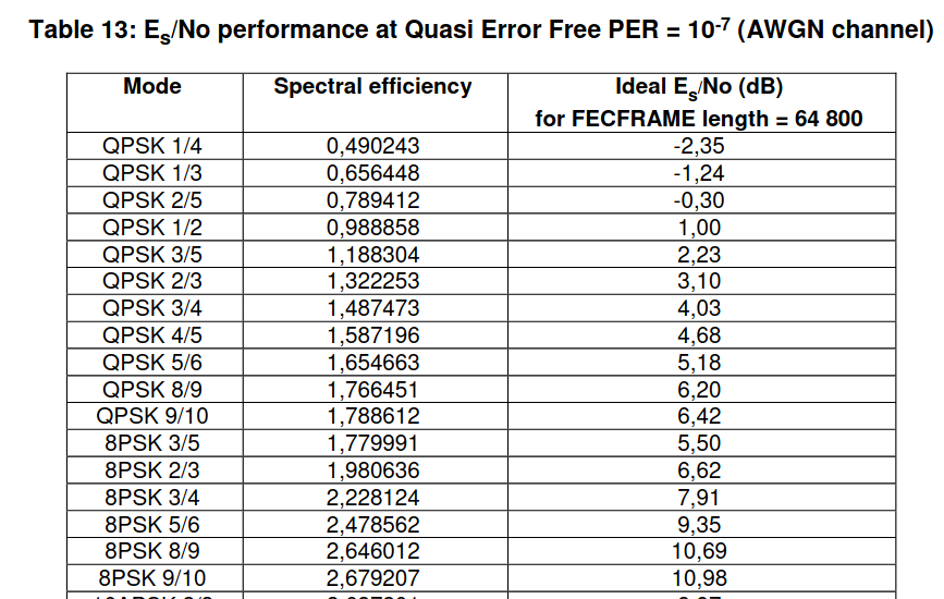
Shannon’s theorem gives a spectral efficiency of 1.42 and 2.26 bits/s/Hz for these two SNRs respectively. Comparing with the DVB-S2 MODCOD table, shown below, appropriate configurations for these SNRs would be QPSK 3/5 for a receiving station like mine, and either 8PSK 3/5 or QPSK 5/6 for a larger receiving station.
For the case in which the beacon is present, due to the gain reduction of 3.5 dB, the beacon now has 67.3 dB·Hz output power. This leaves 71.9 dB·Hz to be used by other stations. Taking into account that the transponder noise floor has been reduced to 65.0 dB·Hz in this case, the SNR would be 1.9 dB·Hz for a station like mine and 5.4 dB·Hz for a station with 6 dB better G/T. The appropriate DVB-S2 MODCODs are now QPSK 1/2 if my station is the receiver, or QPSK 5/6 if the larger station is the receiver.
In this situation, the beacon Es/N0 would be 4.6 dB for a station like mine and 8.6 dB for a station with 6 dB better G/T. Since the beacon uses QPSK 4/5, we see that when the transponder is so busy my station wouldn’t be able to decode the beacon. I have never tested if this is actually true, since I have never found the transponder so busy when I was operating my station (I only operate my station on the WB transponder rarely).
The pie chart for the transponder output power for the 73.8 dB·Hz output power operating point looks like so.
The diagram in terms of PSD is shown here. The area of the rectangles is proportional to power, so their heights are proportional to PSD in linear units. The receiver noise floor is shown for a station like mine. For a station with 6 dB better G/T it would be 1/4 the height, and now comparable to the transponder noise floor.
We see that in comparison with diagram in the previous post, the PSD is much more balanced between the beacon and the other stations. The beacon still has a bit more PSD, but not much. This is the reason why in the SNR budgets computed above the fact that the beacon is present or not does not change the SNR of the other stations by much.
Conclusions
For me, it has been good to reflect on why some of the conclusions of my previous post were wrong. I have already mentioned some of this above. The main mistake was taking 73.0 dB·Hz as the operational point for the output power budget. This actually corresponds to a case in which the transponder is lightly loaded, and is therefore not so relevant. The point of 73.8 dB·Hz used in this post represents a busy transponder much better.
I think that my main mistake was assuming that the data points where the transponder had a 73.8 dB·Hz output power were quite infrequent (which is true), somewhat anomalous (which is not true), and therefore that they should be ignored without looking at these points in more detail to understand why they happen. As it turns out, the transponder is so busy that it reaches this output power quite infrequently. Perhaps for one hour on a weekend evening every other week.
Nevertheless, even though statistically infrequent, it is a relevant scenario. If we count frequency not in terms of time but rather in terms of time multiplied by number of users, then this scenario becomes much more frequent. I guess that some people frequently see the transponder like this, because it’s the only time they have available to operate. When the transponder is less busy, they’re not operating their station.
Another wrong assumption was that going above 73.0 dB·Hz would be too bad in terms of distortion. Looking at what happens in a 73.8 dB·Hz situation, it seems that the distortion is noticeable because the transponder noise floor doesn’t drop as much as the beacon, but it is still quite manageable.
A few comments about going above the 73.8 dB·Hz operating point are in order. First, regarding distortion, one can imagine that distortion will keep growing, so at some point the transponder output power spent in noise and distortion will be the same as when the transponder is “idle”. Increasing the transponder input power even more will only make the distortion worse.
Another disadvantage is the decrease in transponder gain. With the 73.8 dB·Hz operating point, the gain is already 3.5 dB less than with the transponder idle. This means that stations need 3.5 dB more uplink power to obtain the same downlink power than if they were alone in the transponder. Since having a high uplink EIRP is expensive for an amateur station, this sets some practical limits as to what stations can operate when the transponder is so busy.
One of the questions in the previous post was whether the transponder was bandwidth-constrained or power-constrained. There is not a clear dividing line between the two regimes, because there is a continuum of regimes in terms of the maximum spectral efficiency according to Shannon’s theorem. With the reviewed SNRs in this post, we have spectral efficiencies around 1.5 or 2 bits/s/Hz, depending on whether my station or a 6 dB larger one is receiving.
In my opinion, these situations are in the mid-ground between bandwidth-constrained and power-constrained. We don’t have enough bandwidth to use low rate capacity-achieving FEC, but on the other hand, the bandwidth is not so reduced that we need to resort to higher-order modulations such as 16APSK or 32APSK, which come with additional demodulation losses. The range of DVB-S2 MODCODs, between QPSK 1/2 and QPSK 5/6 or 8PSK 3/5 that we’ve seen to be good match for the SNR of the full transponder probably coincide with the MODCODs that people use more often.
Finally, I still feel that the beacon uses too much power (or better said, too much uplink PSD). While it is true that the other stations can manage to achieve the same PSD as the beacon, by doing so the gain of the transponder drops significantly. At this point, smaller stations (and don’t think about my 1.2 m dish here; rather think about an 80cm dish or smaller) can no longer decode the beacon. Also smaller uplink stations are left out of the game by not being able to achieve a downlink signal with reasonable SNR. Using somewhat less uplink PSD (and perhaps somewhat less bandwidth) would perhaps be beneficial, because the gain reduction of the transponder when it is very busy would not be so high as 3.5 dB.
Code
I have updated the Jupyter notebook with the new calculations and plots for this post.
2 comments