Decoding JUICE

JUICE, the Jupiter Icy Moons Explorer, is ESA’s first mission to Jupiter. It will arrive to Jupiter in 2031, and study Ganymede, Callisto and Europa until 2035. The spacecraft was launched on an Ariane 5 from Kourou on April 14. On April 15, between 05:30 and 08:30 UTC, I recorded JUICE’s X-band telemetry signal at 8436 MHz using two of the 6.1 m dishes from the Allen Telescope Array. The spacecraft was at a distance between 227000 and 261000 km.

The recording I made used 16-bit IQ at 6.144 Msps. Since there are 4 channels (2 antennas and 2 linear polarizations), the total data size is huge (966 GiB). To publish the data to Zenodo, I have combined the two linear polarizations of each antenna to form the spacecraft’s circular polarization, and downsampled to 8-bit IQ at 2.048 Msps. This reduces the data for each antenna to 41 GiB. The sample rate is still enough to contain the main lobes of the telemetry modulation. As we will see below, some ranging signals are too wide for this sample rate, so perhaps I’ll also publish some shorter excerpts at the higher sample rate.

The downsampled IQ recordings are in the following Zenodo datasets:

• Recording of JUICE with the Allen Telescope Array on 2023-04-15 (antenna 1a)
• Recording of JUICE with the Allen Telescope Array on 2023-04-15 (antenna 5c)

In this post I will look at the signal modulation and coding, and some of its radiometric properties. I’ll show how to decode the telemetry frames with GNU Radio. The analysis of the decoded telemetry frames will be done in a future post.

Waterfall analysis

First I have computed a waterfall from the IQ recordings and analysed it using the same techniques as for Artemis 1. ATA antennas 1a and 5c were used to record. They have linear polarization feeds. Here I will show the data for antenna 1a. The plots for antenna 5c looks similar and can be seen in the Jupyter notebook.

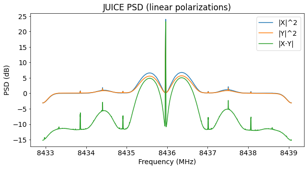
This plot shows the power spectral density in each of the X and Y linear polarizations, and in the cross-correlation between X and Y. The signal is nominally circularly polarized (there seems to be some confusion as to whether it is RHCP or LHCP, and I cannot confirm this because I didn’t calibrate the phase offset between the X and Y channels).

The gain of the two polarization channels has been calibrated using the noise floor outside of the signal. It seems that the two channels have somewhat different system noise temperatures, as the signal power after this calibration is slightly lower in the Y channel.

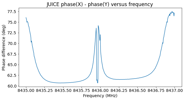
The next plot shows the phase difference between the X and Y channels. We see that this is consistently around 61 deg in the parts of the spectrum where the signal is present. We can use this value to synthesize the circular polarization from the two linear polarization channels.

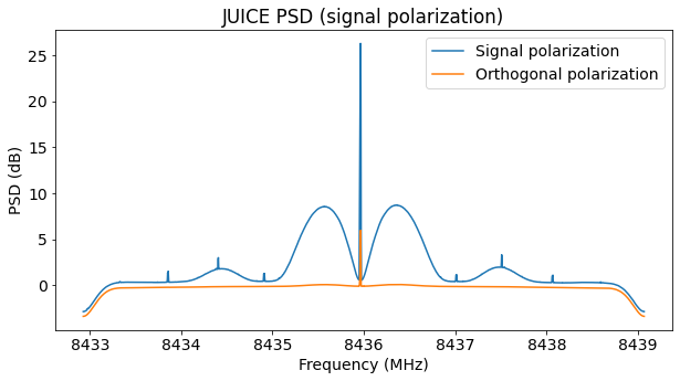
This shows the power spectral density in the signal polarization and in the orthogonal polarization. The polarization synthesis has worked reasonable well, as there is little signal power present in the orthogonal polarization.

Here is the waterfall of the signal polarization, together with an estimate of the CN0 in dB·Hz. We see that there are three distinct regions according to the power of the signal (the low power region appears twice). A small and short drop in signal power near the beginning of the recording should be ignored, because it was caused by a mistake I made with the antenna pointing.

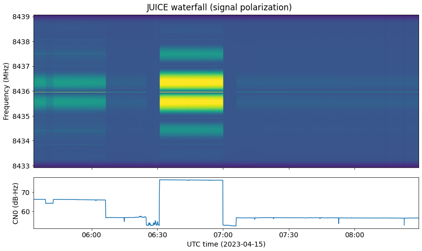
The three power levels that we see are spaced by roughly 10 dB. In fact, the average CN0s that I have measured for these three power levels are 56.4 dB·Hz, 66.0 dB·Hz, and 76.3 dB·Hz. As we will see, there is good evidence that these correspond to three different spacecraft antennas: one of the LGAs (low-gain antenna), the MGA (medium-gain antenna), and the HGA (high-gain antenna). Since this recording was done during the first day of the mission, it is quite reasonable that routine checks were done of all the communications systems. These would involve testing all the spacecraft antennas. In fact, it almost seems that the HGA test was scheduled for 06:30 to 07:00 UTC.

The next figure shows a block diagram of the JUICE RF system. The HGA is a 2.5m dish. The MGA is a 0.5m dish mounted on a steerable boom. Taking into account dish size only, there would be a gain difference of 14 dB between these two antennas. I haven’t found information about the LGAs.

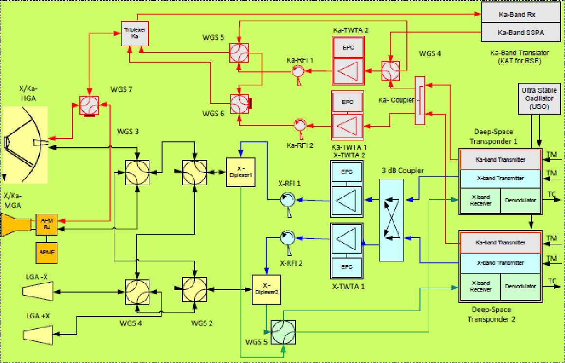
In the block diagram we see that there are two redundant X-band TWTAs and that each of them can be connected to each one of the four antennas via waveguide switches.

The next figure shows the phase difference between the X and Y polarization channels versus time. We see that there are discrete jumps of a few degrees in the phase difference which coincide with the power level changes seen in the waterfall. This is good evidence for the fact that the power changes are caused by the spacecraft switching to a different antenna. Even though all the antennas nominally have the same circular polarization, things are never perfect, so there are small differences between the polarization of different antennas. We can measure these as a change in the phase difference between X and Y. If the power changes where caused only by an output power change, we wouldn’t see any changes in the signal polarization.

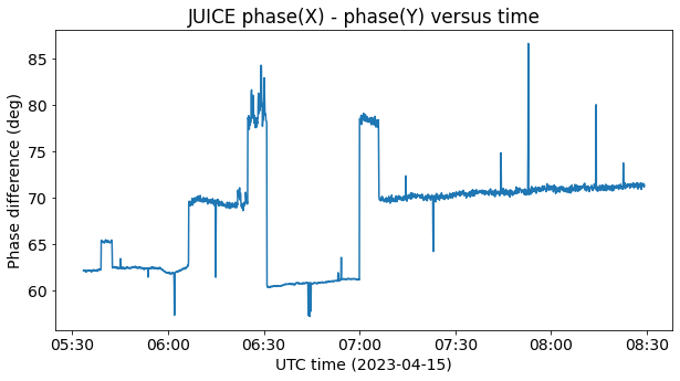
Something else of interest can be seen in this plot. Near the beginning we see a jump in the phase difference, which coincides with my mistake in the antenna pointing. This corresponds to instrumental polarization in the off-axis direction (see this ATA memo for more details).

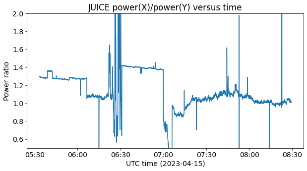
We can also see the same kind of jumps in the power ratio between the X and Y channels.

Modulation and coding

The modulation used by JUICE in this recording is PCM/PM/bi-phase-L. This means that the telemetry data is Manchester encoded and phase-modulated with residual carrier. I have measured a baudrate of 526310.6 baud. Taking into account that the Doppler was almost 10 ppm, this would correspond to a transmit baudrate of approximately 526315.6 baud. I don’t know the reasons behind the choice of this baudrate. The nearest power of 2 is 524288, which is close, but also noticeably different. Perhaps it is related coherently to the carrier frequency.

The coding is CCSDS Turbo coding with r=1/4 and 8920 bit frames. Note that the r=1/4 Turbo code has a small Eb/N0 performance penalty compared to r=1/6, but on the other hand requires less bandwidth. Therefore, it is quite possible that ESA chose r=1/4 as a good trade-off between bandwidth and error-correction performance for this phase of the mission. Most likely they will switch to an r=1/6 Turbo code once the spacecraft is much farther from Earth.

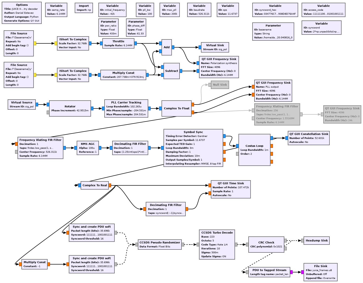
The figure below shows the GNU Radio flowgraph I have used to decode the telemetry. First, circular polarization is synthesized according to the gain and phase corrections computed using the waterfalls. Next, a Rotator block is used to cancel the carrier frequency offset at the beginning of the recording. A PLL is used to lock the residual carrier. I’m using a PLL bandwidth of 100 Hz. The Manchester modulation sideband is dowconverted to baseband, a square pulse shape filter is applied, and the Symbol Sync block with a Gardner TED is used for symbol clock recovery. A Costas loop recovers the residual subcarrier phase and frequency. The Sync and create PDU soft block from gr-satellites performs detection of the ASM (using only the last 64 bits, since that’s the maximum syncword length supported by GNU Radio’s Correlate Access Code block) and extracts PDUs with soft symbols. These are decoded using the Turbo decoder block in gr-dslwp. The Turbo decoder uses 10 iterations for best sensitivity. The FECF (CRC-16) is checked, and correct frames are written to a file.

The following figure shows the GUI of the GNU Radio decoder while processing the beginning of the recording for antenna 1a (this corresponds to the MGA signal).

The Turbo decoder from gr-dslwp is not too fast, so it takes a lot of time to process the complete 3 hour recording. Additionally, the way the ASM (syncword) detection is implemented makes things worse. The CCSDS ASM for r=1/4 Turbo code (and similarly for r=1/6 Turbo) is formed by the concatenation of a 64 bit pattern and the same pattern with all the bits negated. Since we are only using the last 64 bits of the pattern to detect the ASM and also need to try with the ASM and the ASM negated to account for the 180 deg phase ambiguity of the Costas loop, each frame produces a valid ASM detection (corresponding to the second half of the ASM) and an invalid ASM detection (corresponding to the first half of the ASM). All these detections need to go through the Turbo decoder (false detections will be rejected afterwards due to a wrong CRC), so the Turbo decoder workload is doubled. Moreover, the ASM detection allows for up to 16 bit errors (out of 64), which also causes a significant amount of false detections.

Ranging tones

The attentive reader will have noticed a number of CW tones accompanying the signal. These can be seen in the power spectral density plot, which we show again here for convenience.

There are the usual tones produced at even harmonics of the symbol clock. They can be seen in the nulls of the sinc-like shape of the telemetry modulation. They are caused by the pulse shape of the telemetry. A smooth cross through zero of the modulating signal (due to low-pass filtering) causes the residual carrier to increase in power every time that the modulating signal crosses through zero. This causes amplitude modulation in the residual carrier at a frequency equal to twice the symbol clock.

Additionally, there are other CW tones approximately 1.5 MHz away from the residual carrier. They can be seen on top of the third harmonic of the telemetry modulation (which looks like a BPSK sidelobe). Interestingly, these tones are only present when the MGA is used. Perhaps they are present also with the LGA, but too weak to see, but it is clear that they are not present when the HGA is used.

In contrast to the even harmonics of the symbol clock, which are present in the real part of the signal after the PLL, these tones at 1.5 MHz are present in the imaginary part, so they are part of the phase modulation of the X-band downlink. Their exact frequency is very close to \[3\cdot2^{-12}\cdot\frac{221}{749}\cdot7180.151\ \text{MHz}.\]

What’s so significant about this frequency? With a standard X-band turnaround ratio of 880/749, the frequency 7180.151 MHz is the uplink frequency corresponding to a 8435.958 MHz downlink. This is the observed downlink frequency. Note that this downlink frequency includes Doppler, but the beauty of coherent frequency multiplication is that Doppler affects all the involved frequencies by the same multiplicative factor, so we can ignore Doppler for these calculations (the true uplink frequency wouldn’t be 7180.151 MHz, but this value is the “effective” uplink frequency taking two-way Doppler into account). NASA DSN’s 810-005 214 Rev. B Pseudo-Noise and Regenerative Ranging document recommends the following chip rates to be used for PN ranging. These choices are also commonly followed by other agencies, and are in fact standardized by CCSDS (see the Pseudo-Noise (PN) Ranging Systems Blue Book).

The typical values for the parameters \(l_{CR}\) and \(k_{CR}\) are given in the following table.

Thus we see that JUICE is using the \(l_{CR}=12\) and \(k_{CR}=6\), which give a chip rate of approximately 3 Mchip/s and a ranging clock of approximately 1.5 MHz.

Therefore I think that the 1.5 MHz tones we see are the ranging clock of a PN ranging waveform. The ranging session probably ends when the LGA is switched in. The PN ranging waveform would be generated on ground and modulated on the uplink, and then either retransmitted by a spacecraft non-regenerative (bent-pipe) transponder, or demodulated and re-modulated by a spacecraft regenerative transponder.

This paper describes the Ka-band transponder of BepiColombo (apparently the Ka-band transponder of JUICE is very similar), and mentions that it is a regenerative transponder implemented using digital signal processing. I haven’t found any documents confirming that the X-band transponder is also regenerative. It is hard to tell if a transponder is regenerative or not simply by observing the downlink, because the only major difference is that the regenerative transponder gives better SNR because it doesn’t retransmit the uplink thermal noise.

Perhaps in a future post I’ll try to process the PN ranging waveform in this recording.

Two-antenna beamforming

Since the SNR in a single antenna causes a large frame loss when the LGA is used, I have beamformed the two antennas used in the recording to improve the decoding. My approach to beamforming has been to try to keep things as simple as possible. Only the delay between the two antennas is corrected. An independent PLL is used to lock the residual carrier for each of the antennas, and then the outputs of the PLL of each antenna are combined coherently. This saves us from having to adjust the phase of the two antennas, which is a process that needs to be done with an accuracy of a fraction of the carrier wavelength. The correction of the delay between the antennas only needs to be done with an accuracy of a fraction of the wavelength corresponding to the signal bandwidth, so we can do a much coarser correction.

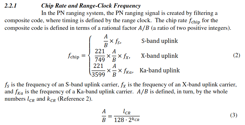
The figure below shows the delay difference (w coordinate, in terms of uvw baseline coordinates) between antennas 1a and 5c during the observation of JUICE. This has been computed using the known ECEF locations of the antennas and the geocentric right ascension and declination coordinates of JUICE taken from HORIZONS (a more careful calculation would take diurnal parallax into account, but this seems good enough). For reference, the signal bandwidth, which is approximately 2 MHz, corresponds to 150 m, and at a sample rate of 6.144 Msps a delay of one sample is 49 m.

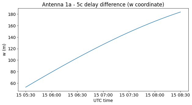
Therefore, we see that we cannot hold a constant delay correction throughout all the recording, since the error at some points would be too large. However, we can model the delay as a linear function, composed by a delay at the beginning of the recording and a delay rate. The next figure shows the difference between the w coordinate and a linear fit to this data. The error is only a few metres.

The delay rate is \(4.082\cdot 10^{-11}\) parts per one. It is tricky to account for this delay rate in GNU Radio because many blocks use float‘s for internal calculations, and this number is significantly smaller than the machine epsilon for a float (we need to use the number 1 plus the delay rate in most calculations).

I have found a rather ugly but effective way of achieving this small delay rate. The Fractional Resampler block can take a float input that specifies the resampling rate for each sample. We can use this block and generate a signal that has a value of one most of the time, and occasionally a slightly larger value (but still representable in a float), such as \(1 + 10^{-6}\) (or actually \(1 + 9.53674\cdot 10^{-7}\), since \(1 + 10^{-6}\) is not exactly representable as a float). By adjusting how often this slightly larger value appears, we can make the average resampling rate equal to \(1 + 4.082\cdot 10^{-11}\). In fact, we achieve this average if the slightly larger value appears once in every 23360 samples. We can easily generate this periodic pattern with a vector source.

Since the Fractional Resampler has an internal delay caused by the MMSE resampler FIR filter that it uses, we include Fractional Resamplers in the signals of the two antennas, but we fix one of them at a constant resampling ratio of one.

The initial delay of 8 samples between the two antennas has been determined by looking at the cross-correlation between the two antennas at the beginning of the recording. Here the plot of the delay difference above is not helpful, because besides the geometric delay difference there are also cable delays that are unknown a priori (in fact note that 8 samples is approximately 392 m, so most of the delay difference is due to cable delays).

The final beamforming decoder flowgraph is shown below. First, for each antenna, the signal polarization is synthesized. Then we have the Delay and Fractional Resampler blocks to correct for the delay difference between the two antennas (including delay rate). Next we have independent PLLs and AGCs. Then, the signals from the two antennas are combined coherently and decoding proceeds as usual.

Software and data

The Zenodo datasets containing the JUICE recording are linked at the beginning of this post. The GNU Radio flowgraphs can be found in this repository. The waterfall and beamforming Jupyter notebooks are here.