In my previous post, I described the observations I had made with the Allen Telescope Array of the Orion vehicle and some of the cubesats of the Artemis I mission following the launch. I showed how to decode the 2 Mbaud OQPSK S-band telemetry signal from Orion using GNU Radio and aff3ct for LDPC decoding. In the post I indicated that I wanted to publish all these recordings in Zenodo, but since I had recorded a large amount of IQ data, I first needed to review the recordings and see what to publish and how to reduce the data.
I have now reviewed the recordings of the Orion 2216.5 MHz signal, and published them in the following datasets:
- Recording of Artemis I Orion with the Allen Telescope Array on 2022-11-16 (part 1/2)
- Recording of Artemis I Orion with the Allen Telescope Array on 2022-11-16 (part 2/2)
Additionally, I have published the decoded AOS Space Data Link telemetry frames in the dataset Decoded Artemis I Orion S-band telemetry frames recieved with the Allen Telescope Array on 2022-11-16.
To review the IQ recordings, I have made waterfalls from the X and Y polarizations of each of the two antennas that I used to record, as well as of the cross-correlation of the X and Y channels of each antenna. This has allowed me to check that the signal polarization stays very consistent throughout the recording. This wasn’t the case with Chang’e 5, which apparently used low gain patch antennas whose polarization depended on the angle from which they were viewed.
Since the polarization doesn’t vary with time, I have replaced the auto-polarization block in the GNU Radio decoder flowgraph by a coherent combination of the X and Y channel using a static phase and amplitude correction for the Y channel. This has improved the number of decoded frames. I originally designed the auto-polarization algorithm for a signal having a residual carrier and no interference. I think that the algorithm wasn’t behaving too well with the Orion wideband signal, specially when signals from other satellites appeared in the passband (which happens a few times).
As the polarization synthesis using static parameters has worked quite well, I have decided to publish the data with the polarization synthesis applied. This cuts the data size in half, because we can publish only the signal polarization instead of the X and Y channels. Additionally, as the dynamic range of the signal is not large, I have reduced the number of bits from 16 to 8. This already gives sizes which are manageable to publish in Zenodo.
I used two antennas, 1a and 5c, to record. However, since the SNR in a single antenna is already quite high, I have decided to publish the data for only one antenna. This is antenna 1a, which has a slightly higher SNR than antenna 5c and is also the antenna that I used in the previous post and in the analysis below.
The waterfalls are obtained with the GNU Radio flowgraph artemis_waterfall.grc, which is shown below. This flowgraph computes the FFTs of the two polarizations of each antenna and integrates the power of each polarization and their cross-product. The results are written to files.
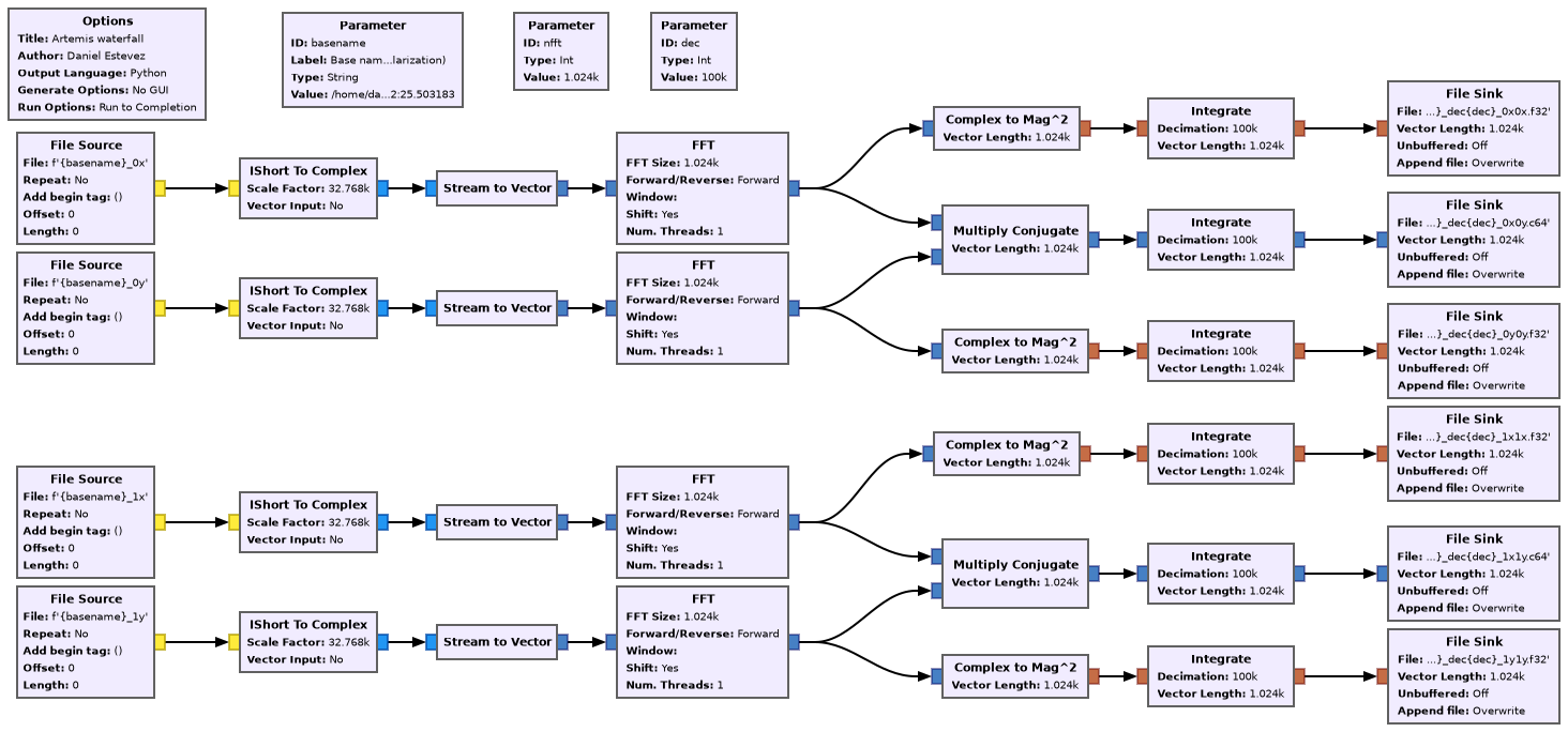
The output of this flowgraph is analyzed in this Jupyter notebook, which produces some plots related to each waterfall. The current version in the repository also shows the waterfalls for the cubesat LunaH-Map (known as HMAP by the DSN). The X-band telemetry of this cubesat will be the topic for the next post in the Artemis I series.
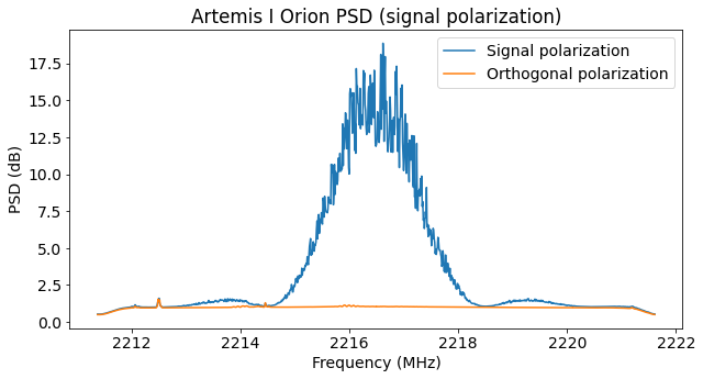
The figure below shows the power spectral density in the signal polarization and the orthogonal polarization. The leakage of the Orion signal into the orthogonal polarization is imperceptible, which means that our polarization synthesis is working quite well.
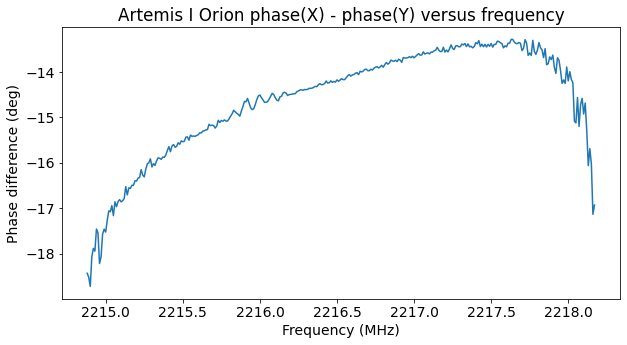
To assess further the quality of the polarization synthesis, it is convenient to plot the phase difference between the X and Y channels versus frequency and versus time. In the plot of phase difference versus time we can see a small slope on the order of 3 degrees in 3 MHz. This corresponds to a small delay difference between the X and Y channels, most likely caused by slightly different cable lengths. The corresponding delay is 2.8 ns, or 80 cm. Since the delay difference is small, we do not need to correct it.
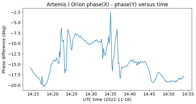
In the plot of phase difference versus time we see variations on the order of 10 degrees. These are perhaps due to instrumental polarization in the ATA antennas. Since I was tracking “by hand” using a manually determined n offset from a TLE in order to maximize the signal power, there would be a pointing error that changes with time. The sudden jumps in the plot could then correspond to the moments in which I updated the antenna pointings (the antennas were made to track a fixed right ascension and declination, which I kept updating). Another possible explanation for the changes in phase difference is that the signal polarization actually changed slightly. Orion made the first orbital manoeuvering system burn at 14:33 UTC, so perhaps the sudden jumps that appear correspond to the the spacecraft changing attitude.
The figure below shows the waterfall corresponding to the signal polarization, together with the estimate of the signal CN0. There are a few drops in signal power that match the jumps in the plot of phase difference shown above. The CN0 is around 74 dB·Hz. This corresponds to an EbN0 of 11 dB, which is more than enough for error-free decoding of r=1/2 LDPC.
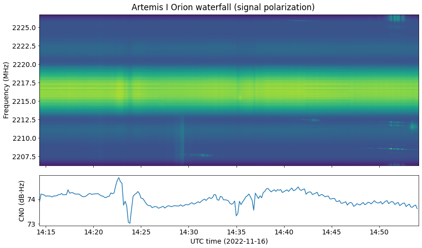
In the waterfall we can see signals from other satellites. These are most likely LEO satellites whose signals enter through the sidelobes of the antenna. The sidelobes of the ATA antennas are relatively strong.
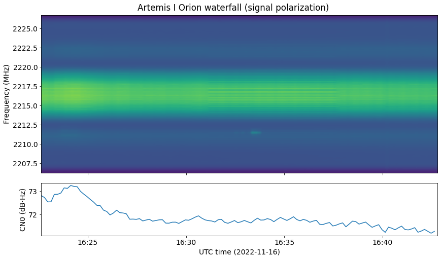
The next figure shows the waterfall of the second recording. The signal is slightly weaker, but there are no sudden changes in signal power.
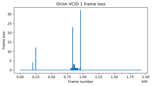
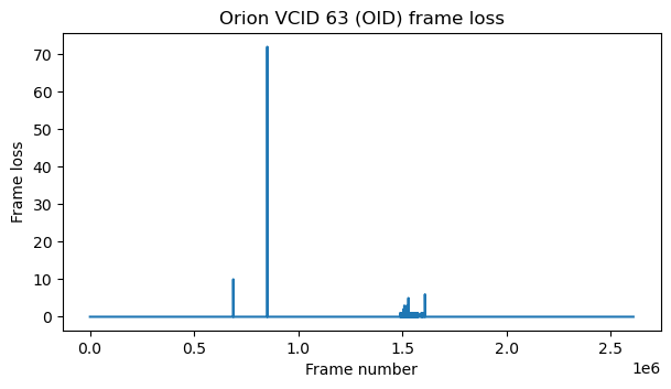
I have re-run the decoder for the Orion S-band telemetry using the static polarization synthesis parameters derived from these waterfalls. The results have greatly improved for the 14:14 UTC recording, in which 77277 were lost on my first decoding attempt. Now the number of lost frames has decreased to 698. In the 16:22 UTC recording the number of lost frames has changed from 103 to 128.
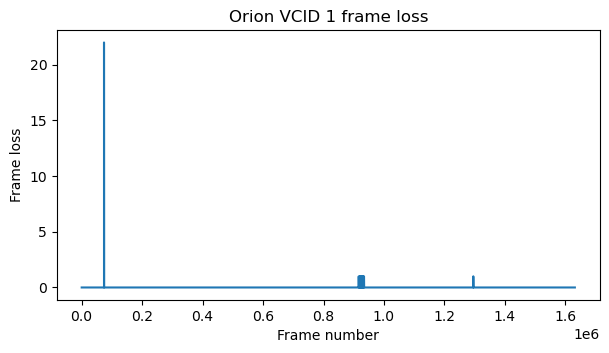
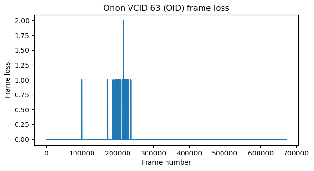
The figures below show the number of lost frames in each virtual channel in the 14:14 UTC recording. These can be compared to the corresponding plots in the previous post.
The plots for the 16:22 UTC recording are the following.
Code and data
The Jupyter notebook for the analysis of the Orion frames, as well as the OQPSK demodulator flowgraph, have been updated in this repository. The flowgraph and notebook for the waterfall plots can be found in my ata_notebooks repository. The links to the datasets in Zenodo are listed at the beginning of the post.
3 comments