Decoding Euclid

Euclid is an ESA near-infrared space telescope that was launched to the Sun-Earth Lagrange L2 point on July 1, using a Falcon 9 from Cape Canaveral. The spacecraft uses K-band to transmit science data, and X-band with a downlink frequency of 8455 MHz for TT&C. On July 2 at 07:00 UTC, 16 hours after launch and with the spacecraft at a distance of 167000 km from Earth, I recorded the X-band telemetry signal using antennas 1a and 1f from the Allen Telescope Array. The recording lasted approximately 4 hours and 30 minutes, until the spacecraft set.

Even though the telemetry signal fits in about 300 kHz, I recorded at 4.096 Msps, since I wanted to see if there were ranging signals at some point. Since the IQ recordings for two antennas at 4.096 Msps 16-bit are quite large, I have done some data reduction before publishing to Zenodo. I have decided to publish only the data for antenna 1a, since the SNR in a single antenna is already very good, so there is no point in using the data for the second antenna unless someone wants to do interferometry. Since looking in the waterfall I saw no signals outside of the central 2 MHz, I decimated to 2.048 Msps 8-bit. Also, I synthesized the signal polarization from the two linear polarizations. To fit within Zenodo’s constraints for a 50 GB dataset, I split the recording in two parts of 32 GiB each.

The recording is published in these two datasets:

• Recording of Euclid with the Allen Telescope Array on 2023-07-02 (part 1/2)
• Recording of Euclid with the Allen Telescope Array on 2023-07-02 (part 2/2)

In this post I will look at the signal modulation and coding and present GNU Radio decoders. I will look at the contents of the telemetry frames in a future post.

Finding Euclid

Before jumping on to the signal analysis, I think it is good to say a few words about how we found Euclid. Usually, ephemerides for deep space launches, specially those of “western” space agencies will be released publicly ahead of time. The typical places where this is done are NASA JPL Horizons, which allows to calculate spacecraft positions and other data for different observers and times with a web interface, and, for the case of ESA, the ESA SPICE service, which doesn’t have such an easy to use interface, but allows anyone handy with the SPICE Toolkit to run the calculations on their own using the SPICE kernels that are published in the repository.

Publishing the ephemeris is seen as common procedure and good practice because it enables other scientists to use the spacecraft as a target of opportunity (for example to try to observe it with optical telescopes) and for general space situational awareness.

In the case of Euclid, to this date I have not seen any official public trajectory data for the spacecraft, in contrast to what has happened with other launches, including JUICE, which is ESA’s previous deep space launch. Some people suspect that this is for security reasons, but I think that perhaps the reason is a simple as the proper channels and procedures to release the data being missing.

Not having ephemerides for a spacecraft is annoying, because it makes it tricky to find it on the sky. The larger the antenna on the groundstation, the narrower the beamwidth, and the more time consuming that it is to search a region of the sky. However, the amateur spacecraft observer community has shown repeatedly to be quite good at this task. Stations with smaller antennas can find the spacecraft relatively easily when it is still near Earth, and provide pointing data for larger stations, which in turn are able to get more precise pointing data to derive a better orbit estimate. This happened 3 years ago with Tianwen-1, and has also happened now with Euclid and other launches. I think this shows the readiness and technical skill of the community, and that not publishing ephemerides for security reasons is rather pointless.

When Euclid launched, Jonathan McDowell created a TLE and state vector basically by looking at the graphics and data in the SpaceX livestream. Then Edgar Kaiser DF2MZ found the signal with his small station. This allowed other several other stations in Europe, and later in North America to find Euclid as well. Using the pointing data from Jean-Luc Milette‘s 4 metre dish at 02:40 UTC, I was able to find it with the ATA 6 metre dishes at 07:00 UTC without too much effort.

The pointing I used with the ATA was a constant correction of -1.58 deg in RA and 0.04 deg in DEC applied to the ephemerides I had made by propagating Jonathan’s state vector in GMAT. I have now seen that Project Pluto has some ephemerides for Euclid (possibly derived from optical observations), but I don’t know if these were available earlier.

Waterfall analysis

As in other observations with the ATA, I have first done an analysis of the waterfalls of the recordings. The code I have used is the same as for the JUICE observation. The following plots correspond to antenna 1a.

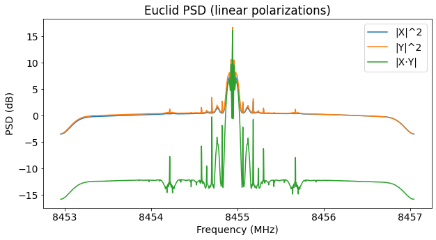
This figure shows the power spectral density in the linear polarizations X and Y, as well as their cross-correlation. The gain calibration for each channel has been done using the noise floor as reference. As we expect for a circular polarization, the signal has the same power in the X and Y channels, and also in the cross correlation.

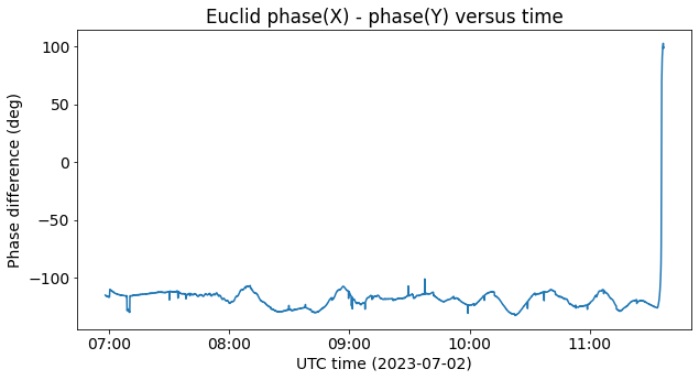
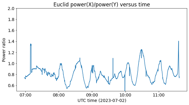
The phase difference and power ratio between the X and Y channels stay roughly constant throughout all the recording until the moment when the signal is lost as Euclid sets below the 16.8 degree elevation mask for the antenna tracking.

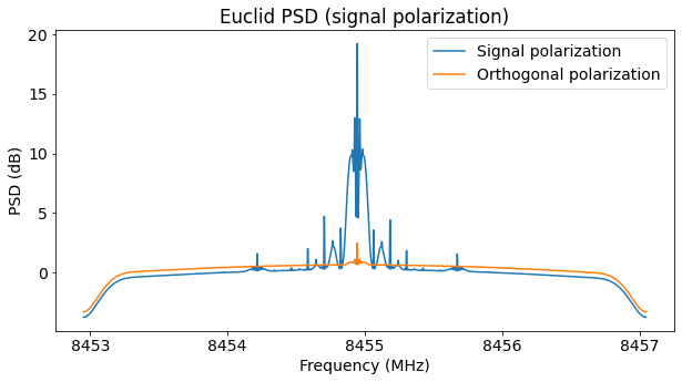
Using the average of the phase difference and the power ratio, we can synthesize the signal polarization. As shown below, all of the signal is present in this polarization, except for a small amount of power that leaks to the orthogonal polarization.

The following shows the waterfall of the signal together with an estimate of its CN0. The CN0 stays roughly constant at a value around 61.9 dB·Hz. The waterfall for antenna 1f looks similar, but the SNR is slightly lower. For this reason, I have decided to publish only the data of antenna 1a. The CN0 is so steady that the changes in antenna pointing every 10 minutes are clearly visible.

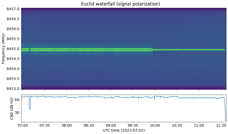
The drop in signal power at around 07:10 UTC corresponds to a mistake I did in the antenna pointing. We can see a change in modulation just before 10:00 UTC. The waterfall of the part 2 recording in Inspectrum gives more details about this event. The spacecraft receives a telecommand, which we can see in the telecommand loopback. Three seconds later, the telemetry modulation stops. The transponder is still working, as we still see the telecommand idle signal in the loopback. In fact, as the telemetry modulation has been removed, the loopback has increased in power.

About three seconds later, the telemetry modulation resumes at a lower rate.

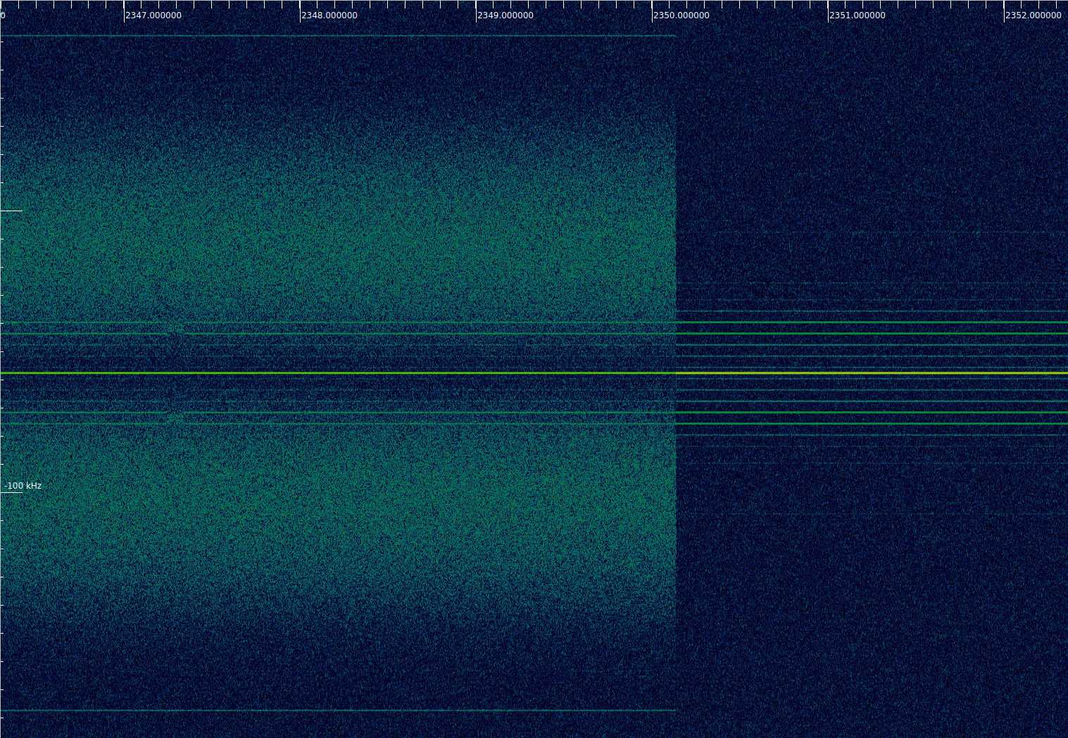
Some time after the modulation change there is a groundstation hand-over. The first groundstation (probably Malargüe, in Argentina) loses lock, and the second groundstation (probably New Norcia, in Australia) acquires lock afterwards. We can first see that telecommand modulation stops, and a fraction of a second later the carrier unlocks and jumps slightly in frequency.

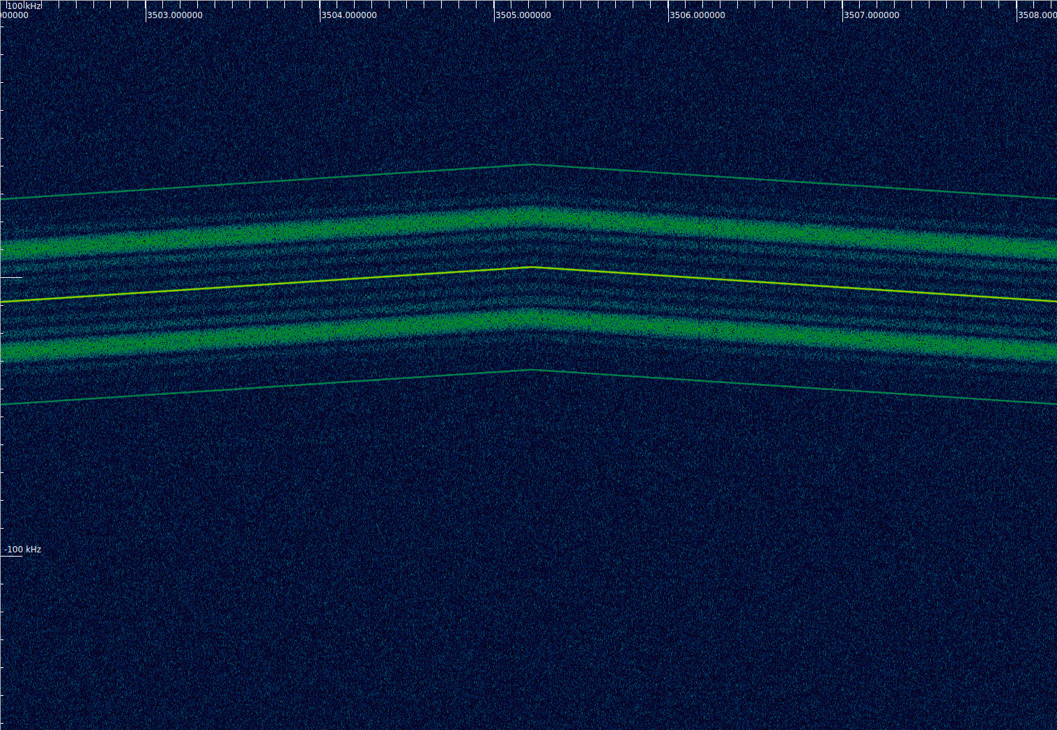
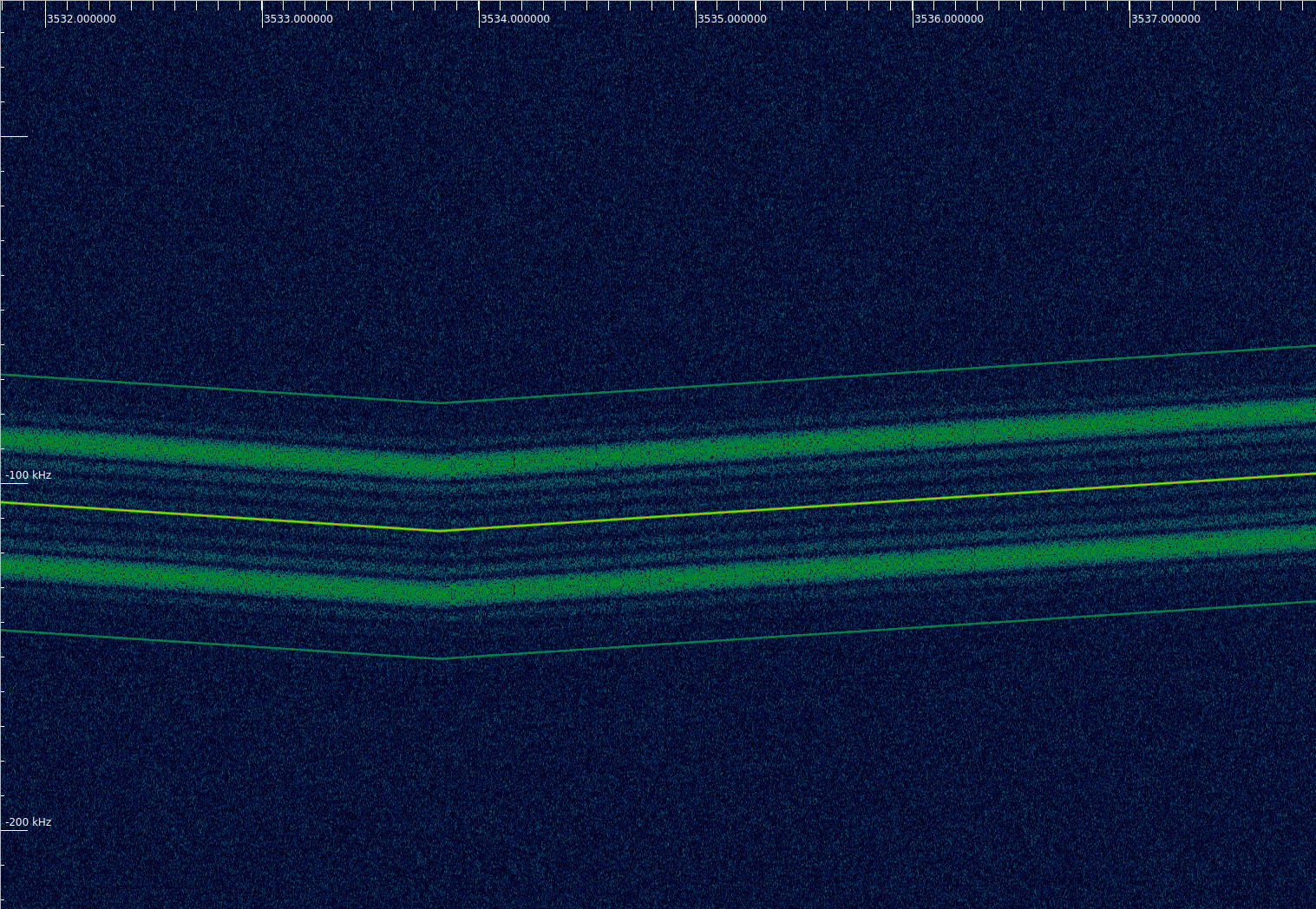
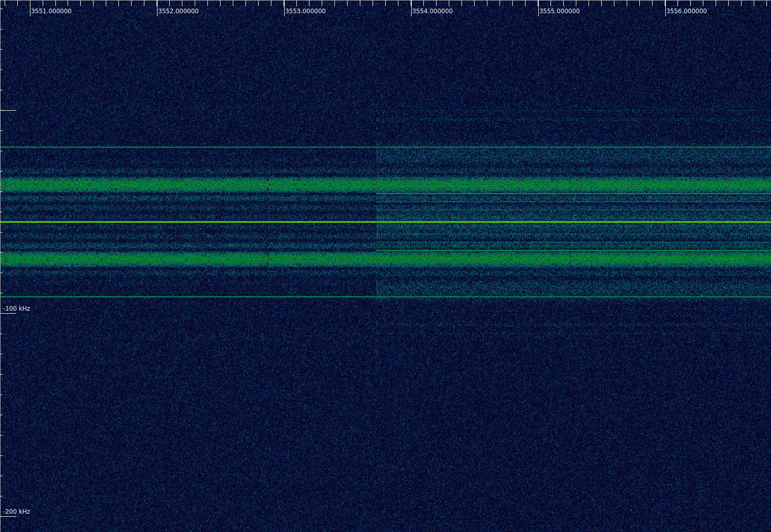
The downlink is non-coherent for 57 seconds, and then it jumps in frequency as it locks to the new uplink carrier, which is sweeping up.

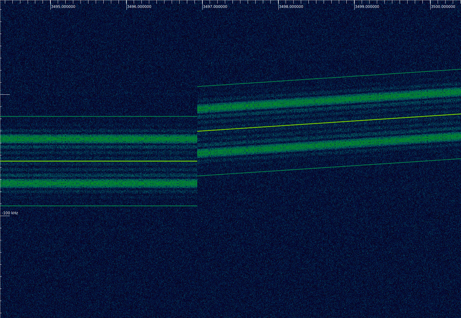
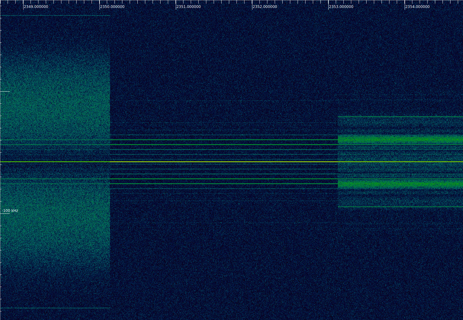
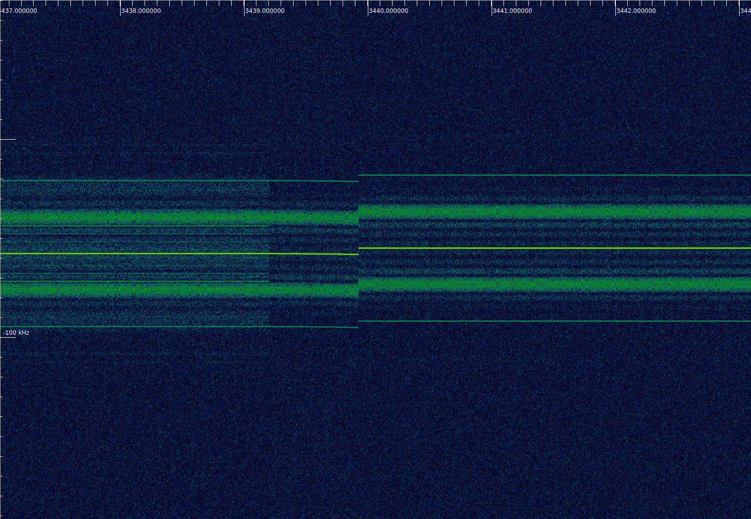
The sweep continues describing the following pattern:

• 3497 seconds. -30 kHz. Lock
• 3505 seconds. 3 kHz. Top of the sweep
• 3534 seconds. -113 kHz. Bottom of the sweep
• 3548 seconds. -55 kHz. End of the sweep

Therefore, we see that the sweep is done at a rate of 4 kHz/s over a total span of 116 kHz. The sweep begins upwards, reaching the top of the sweep, then continues downwards until reaching the bottom, and finally goes upwards again, settling at the midpoint between the top and bottom frequencies. The key moments of the sweep are shown in the next figures.

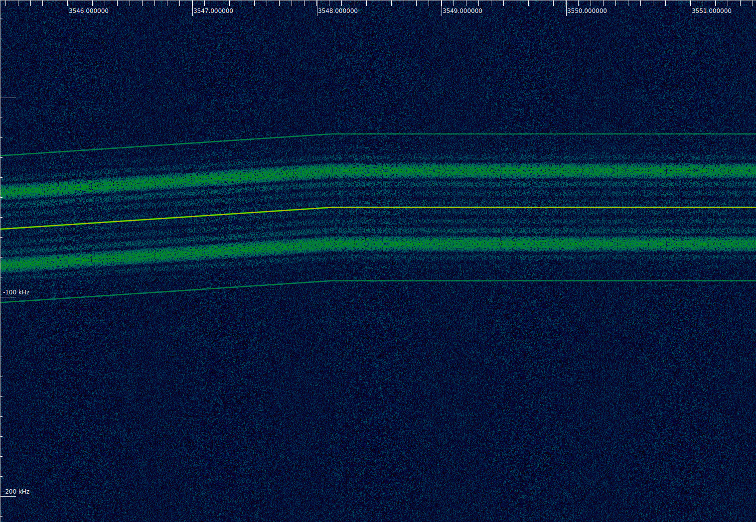
The telecommand modulation is started approximately 5 seconds after the end of the sweep.

Modulation and coding

We have seen Euclid using two different modulations. They are PCM/PM/bi-phase-L at 59879.8 baud (Manchester modulation with residual carrier), and PCM/PSK/PM at 4606 baud (subcarrier modulation with residual carrier) with a subcarrier frequency of 18424.5 Hz (4 times the baudrate). These are the values I have measured from the recording. The nominal values are maybe 60 kbaud (or 59.9 kbaud) and 4.6 kbaud respectively, although other ESA spacecraft use baudrates which are not nice round numbers.

The coding in both modes is the same: CCSDS concatenated coding using Reed-Solomon with an interleaving depth of 5. This means that the codewords are 1275 bytes long and contain 1115 information bytes when decoded. A FECF (CRC-16) is present at the end of the frames.

This paper mentions that Euclid supports two telemetry rates on X-band: 2 kbps and 26 kbps. Taking into account the concatenated coding overhead, the baudrates we have seen give data rates which are pretty close to these values (4.6 kbaud gives 2005.1 bps and 60 kbaud gives 26153.2 bps). Therefore, it seems that this recording is a good example of the two telemetry modulations supported by Euclid.

There is something unusual about the 2 kpbs modulation, which is that the telecommand loopback with a 16 kHz subcarrier falls on top of the telemetry subcarrier. This is not so good, because the telecommand loopback causes a certain amount of interference in the telemetry decoder, as we will see. I don’t know why such a low telemetry subcarrier frequency has been chosen. It is much more common to choose a subcarrier frequency well above 16 kHz to leave room for the telecommand loopback.

GNU Radio decoder

I made a GNU Radio decoder for the 26 kbps modulation before observing with the ATA. Paul Marsh M0EYT did some recordings of Euclid on the UTC evening of July 1, when the spacecraft was first visible over Europe. Using those recordings, I quickly prepared a GNU Radio decoder, which can be found here. The GNU Radio decoder I used for the 26 kbps modulation in the ATA recording is a small adaptation of this one, and the 2 kbps decoder is also based on it.

The flowgraph for the 26 kbps signal can be found here. It is a typical PCM/PM/bi-phase-L demodulator followed by the gr-satellites CCSDS Concatenated Deframer block.

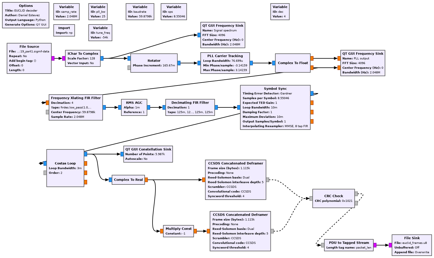
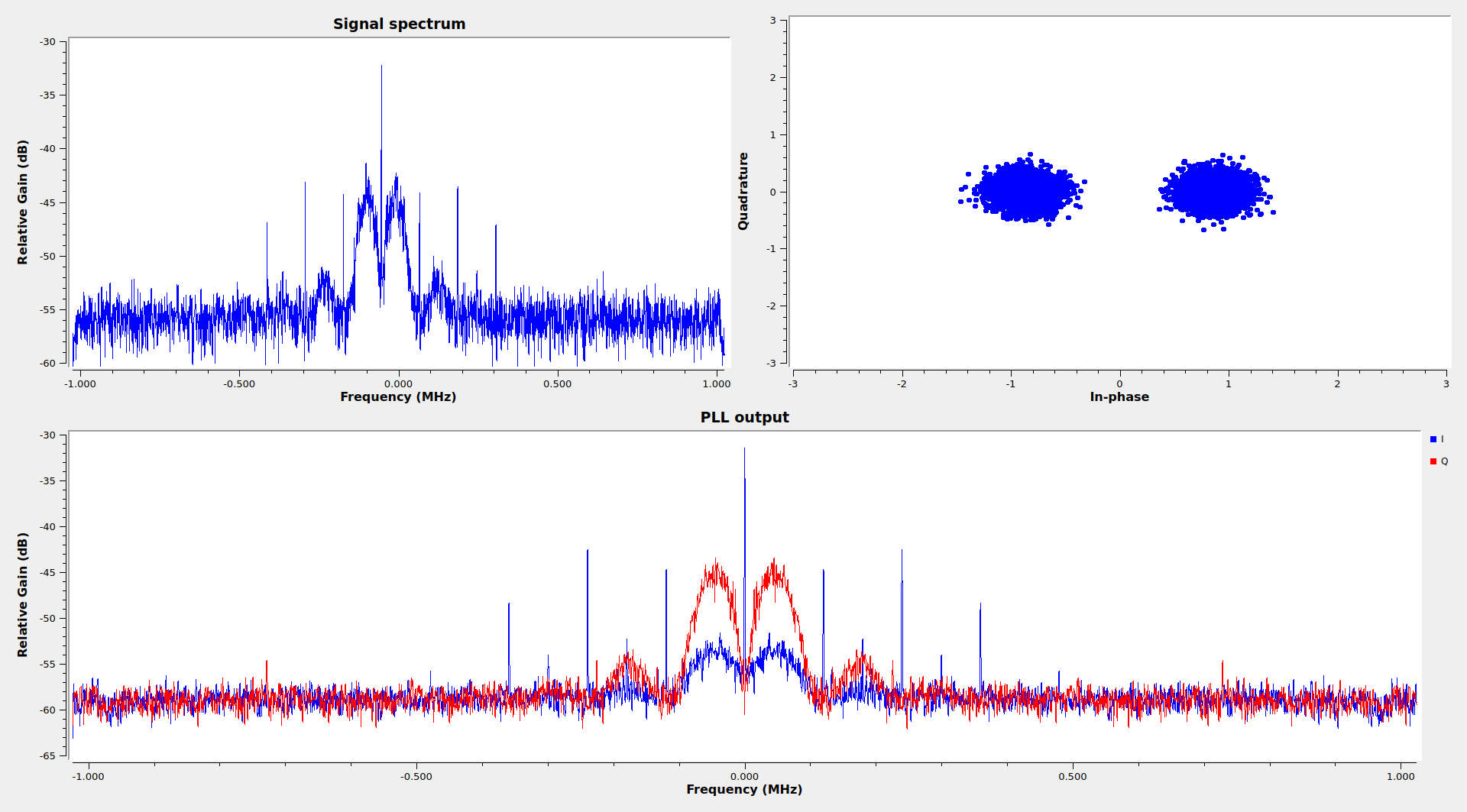
The GUI of the flowgraph running on the ATA recording is shown here.

The 2 kbps flowgraph is very similar to the previous one. The only difference is the subcarrier frequency and symbol rate. I have also added a section at the bottom of the flowgraph to measure the phase of a ranging tone at a frequency of 728.2 kHz (described below in more detail).

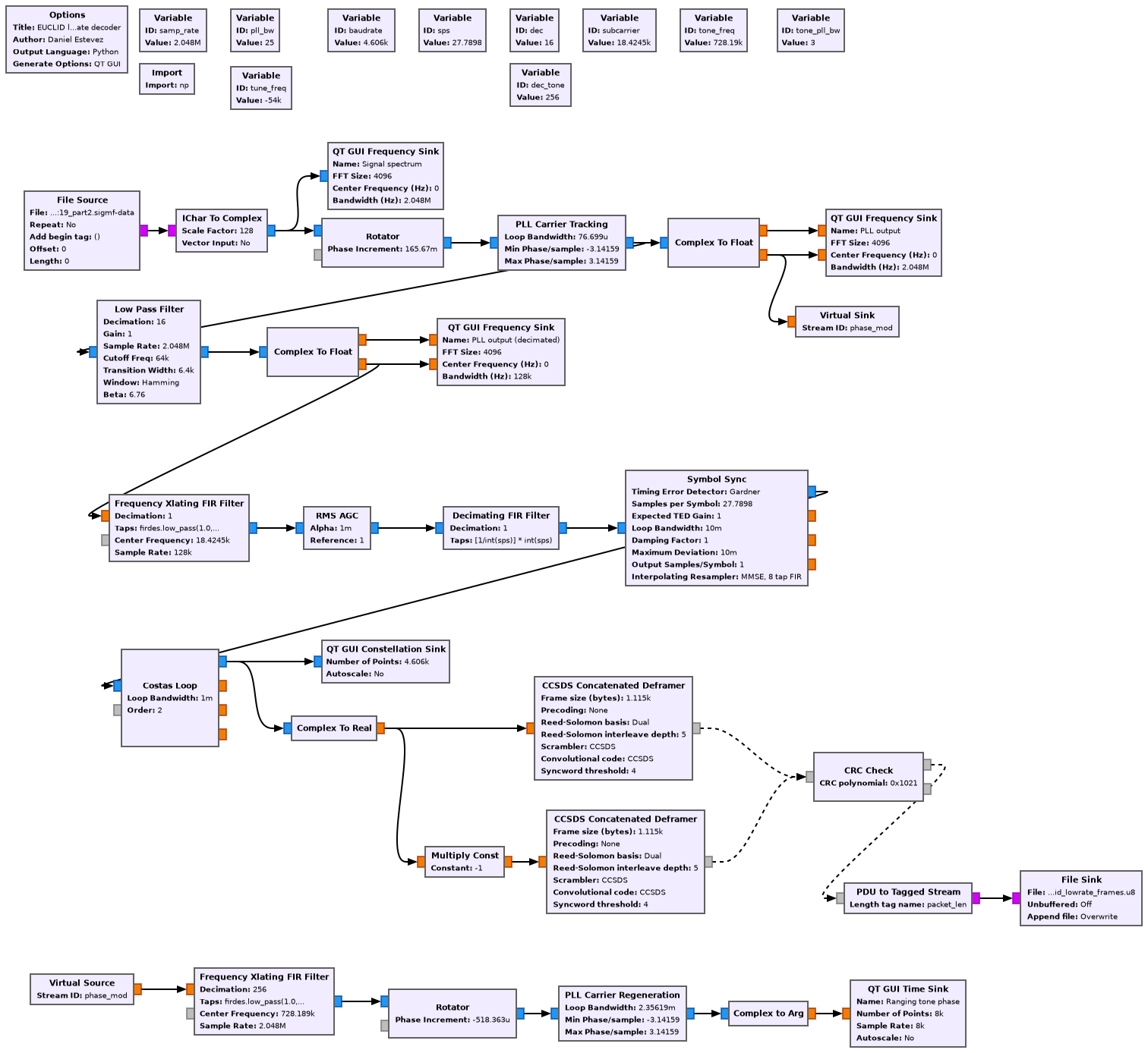
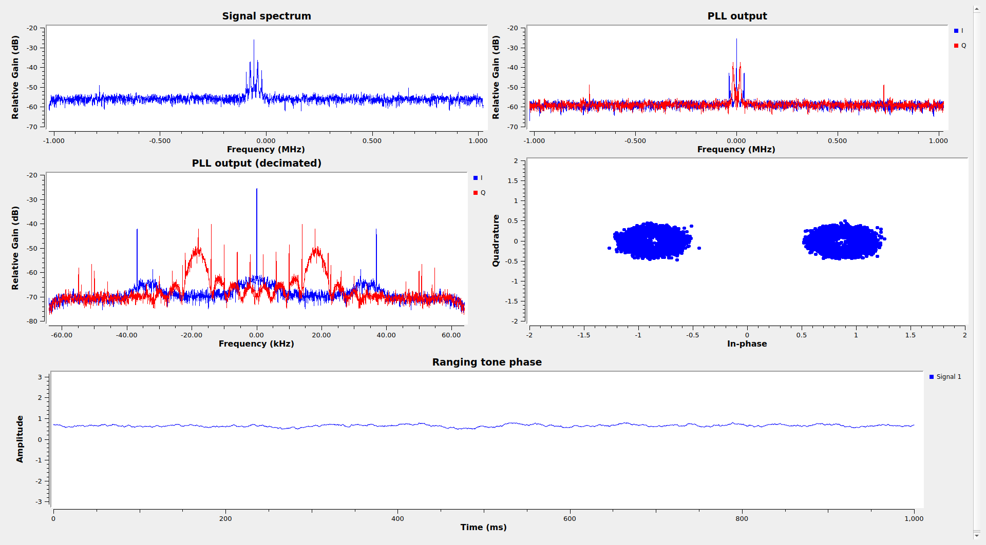
The GUI of this flowgraph running on the 2 kbps signal is shown here. The interference of the telecommand signal on the telemetry subcarrier is apparent. We see in the spectrum that one of the telecommand idle signal tones falls in the middle of the telemetry signal. This causes a constellation that looks like a pair of rings, instead of two points.

Ranging signals

As I mentioned above, there is a tone at +/- 728.2 kHz from the residual carrier that got my attention. The tone is stronger in the 2 kbps modulation, but it is also present in the 26 kbps modulation. At the output of the PLL the tone is on the imaginary part, which means that it is part of the phase modulation of the downlink carrier.

This tone is present since the beginning of the recording, but disappears at second 3355 in part 2, which is 84 seconds before the first groundstation unlock. The tone reappears at second 3627, which is 73 seconds after the second groundstation has started the telecommand modulation.

Another clue of the nature of this tone is present during the modulation change. When the telemetry modulation stops, the power of the tone increases, in the same way that the power of the telecommand loopback also increases. When the 2 kbps modulation starts, the power of the tone decreases slightly, as it also happens to the telecommand loopback. This means that the tone is an uplink signal that is turned around by the transponder.

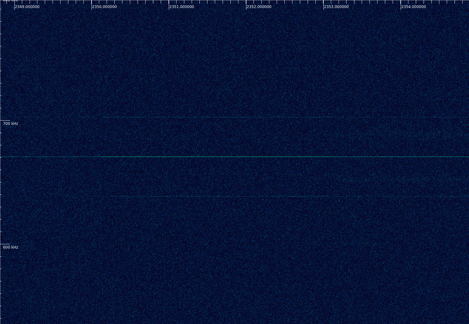
The exact frequency of this tone at a certain moment when I decided to measure it is 728189.66 Hz (the frequency of the tone changes with Doppler, and is probably coherent to the uplink frequency).

This is most likely a ranging signal, but I am not sure of which type of ranging signal. I have considered that it could be the ranging clock of a PN ranging signal. However, its frequency does not match the formula of recommended chip rates in the CCSDS Blue Book. I have also noticed that there are two weaker tones around this signal. They are 32 kHz away from it. It might be the case that the stronger tone at 728.2 kHz plus the weaker tones at +/- 32 kHz offset are the complete ranging signal. The +/- 32 kHz tones would provide ambiguity resolution (~4.7 km of one-way range), and the 728.8 kHz main tone would be used for precise measurement. If the auxiliary tones are able to give the ambiguity resolution that is required, then certainly this ranging signal is simpler and more effective than sequential ranging or PN ranging.

Telecommand modulation

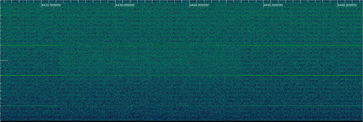
The telecommand modulation is the standard 4 kbaud PCM/PSK/PM with a 16 kHz subcarrier. Most of the time the telecommand signal is idle, producing tones at +/- 2 kHz from the subcarrier frequency. Occasionally there are some telecommand frames. There are a few before the change to the 2 kbps modulation. It is also noteworthy a 25 second segment starting at 4422 seconds in the part 1 recording, in which many telecommands are sent. This figure shows the telemetry subcarrier decimated to 16 ksps in Inspectrum. Telecommands are best seen by the interruption of the idle tones.

Code and data

The links to the IQ recording in Zenodo are given at the beginning of the post. The GNU Radio flowgraphs can be found in this repository. The waterfall plots have been done in this Jupyter notebook.