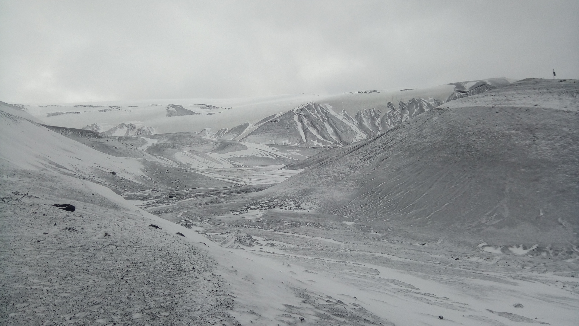
As you may know, between January 14 and February 18 I have been away from home on a research expedition to Antarctica. Several people have asked me for a post detailing my experiences, and I was also thinking to write at least something about the trip. I could spend pages talking about the amazing landscapes and fauna, or daily life in Antarctica. However, in keeping with the spirit of this blog, I will concentrate on the radio related aspects of the trip (and there are indeed enough to tell a story). If I see that there is much interest in other topics, I might be persuaded to run a Q&A post or something similar.
Apparently, my trip and my posts in Twitter raised the attention of a few Hungarian Amateurs, who even discussed and followed my adventures in their Google group. Thanks to Janos Tolgyesi HG5APZ for his interest and for some good discussion over email during my voyage.
However, so far the reflection has been detected by hand by looking at the recording waterfalls. We don’t have any statistics about how often it happens or which conditions favour it. I want to make some scripts to process all the Dwingeloo recordings in batch and try to extract some useful conclusions from the data.
Here I show my first script, which computes the power of the direct and reflected signals (if any). The analysis of the results will be done in a future post.
I have already spoken about the Moonbounce signal from DSLWP-B in several posts. To sum up, DSLWP-B is a Chinese satellite that is orbiting the Moon since May 25. The satellite has an Amateur payload that transmits GMSK and JT4G telemetry in the 70cm Amateur satellite band. This signal can be received by well equipped groundstations on Earth, including the 25m radiotelescope at Dwingeloo, in the Netherlands (and also by much smaller stations).
The people at Dwingeloo publish the recordings that they make of the RF signal. In two of these recordings, the signal from DSLWP-B is received not only via the direct path, but also through a reflection off the Moon’s surface. The reflected signal is around 25dB weaker, usually has a different Doppler shift, and has a Doppler spread of around 50 to 200Hz.
What I find most interesting about this is that of all the days that Dwingeloo has observed DSLWP-B, in only two of them (on 2018-10-07 and 2018-10-19) the Moonbounce signal has been visible. Mathematically, using a specular reflection on a sphere model, whenever the satellite is visible directly, there is also a ray from the spacecraft that reflects off the lunar surface and arrives at the groundstation (see the proof here). Therefore, I think that there must be something about the particular geometry of the days 7th and 19th that made the Moon reflections relatively stronger and hence detectable. Here I use GMAT to study the orbital geometry when the reflections were received.
On the other hand, JT4G is a digital mode designed for Earth-Moon-Earth microwave communications, so it is tolerant to high Doppler spreads. However, the reflections of the B0 transmitter at 435.4MHz, which contained the JT4G transmissions, were very weak, so I had not attempted to decode the JT4G Moonbounce signal.
On 2018-10-19, the Moonbounce signal from DSLWP-B was again visible in Dwingeloo’s recordings. I have used the 2018-10-19T17:53:35 435.4MHz recording and managed to decode the Moonbounce signal of one out of the five JT4G transmissions that appear in the recording.
To extract the data from the recording to WAV files that can be read by WSJT-X, I have used the following Jupyter notebook. Then I have used WSJT-X version 2.0.0-rc3 to try to decode the Moonbounce signal. Since the JT4 decoder only decodes a single signal at the selected frequency, it is enough to select the frequency of the Moonbounce signal in WSJT-X. The direct signal will not be decoded, even though it is also present in the WAV file.
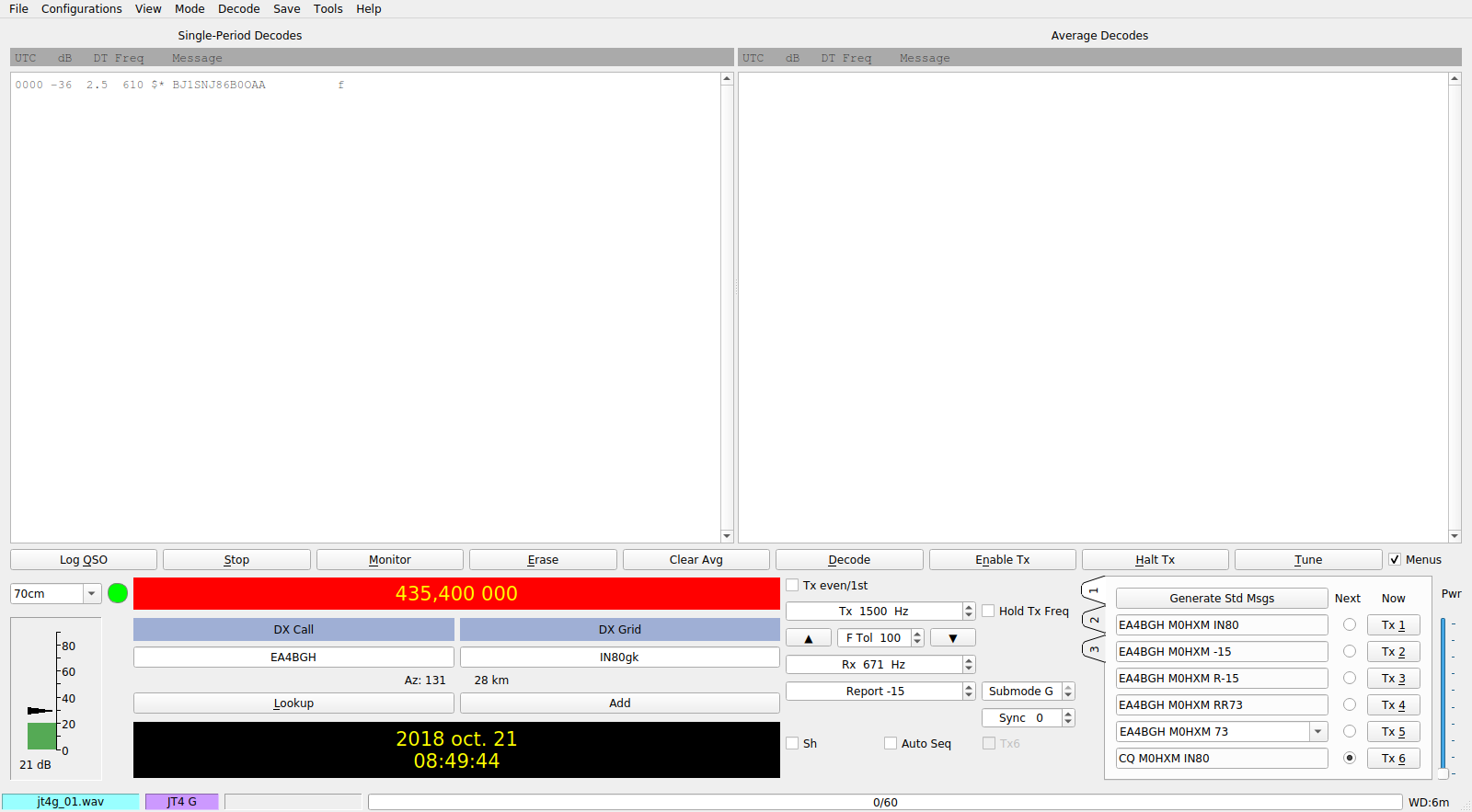
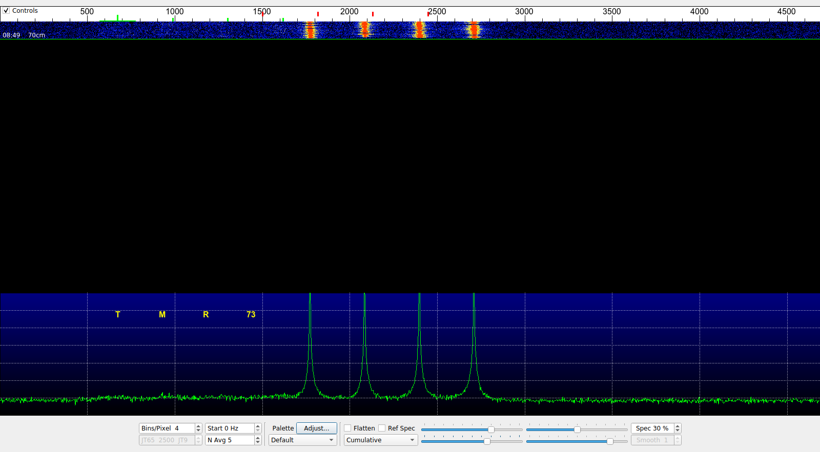
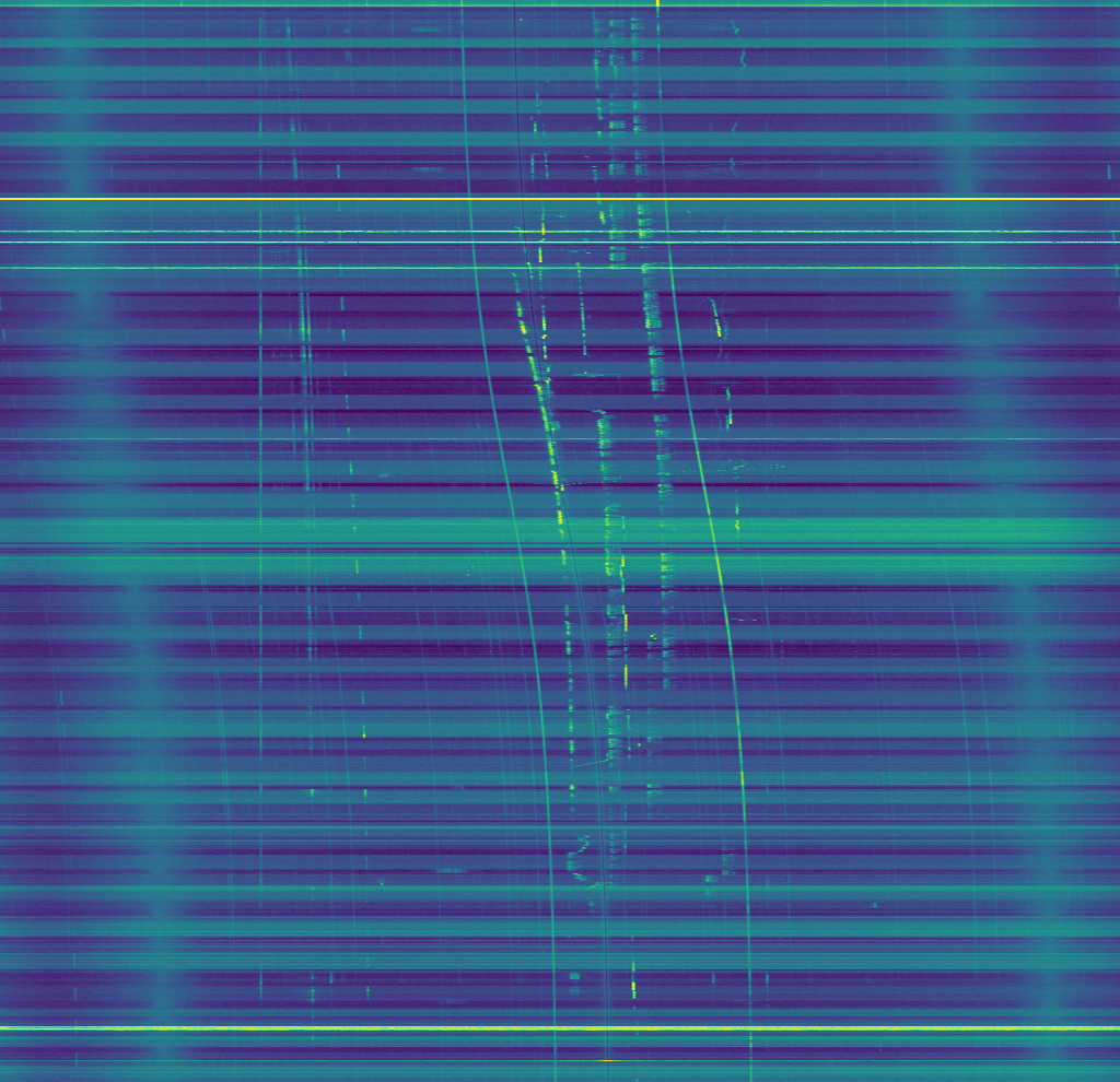
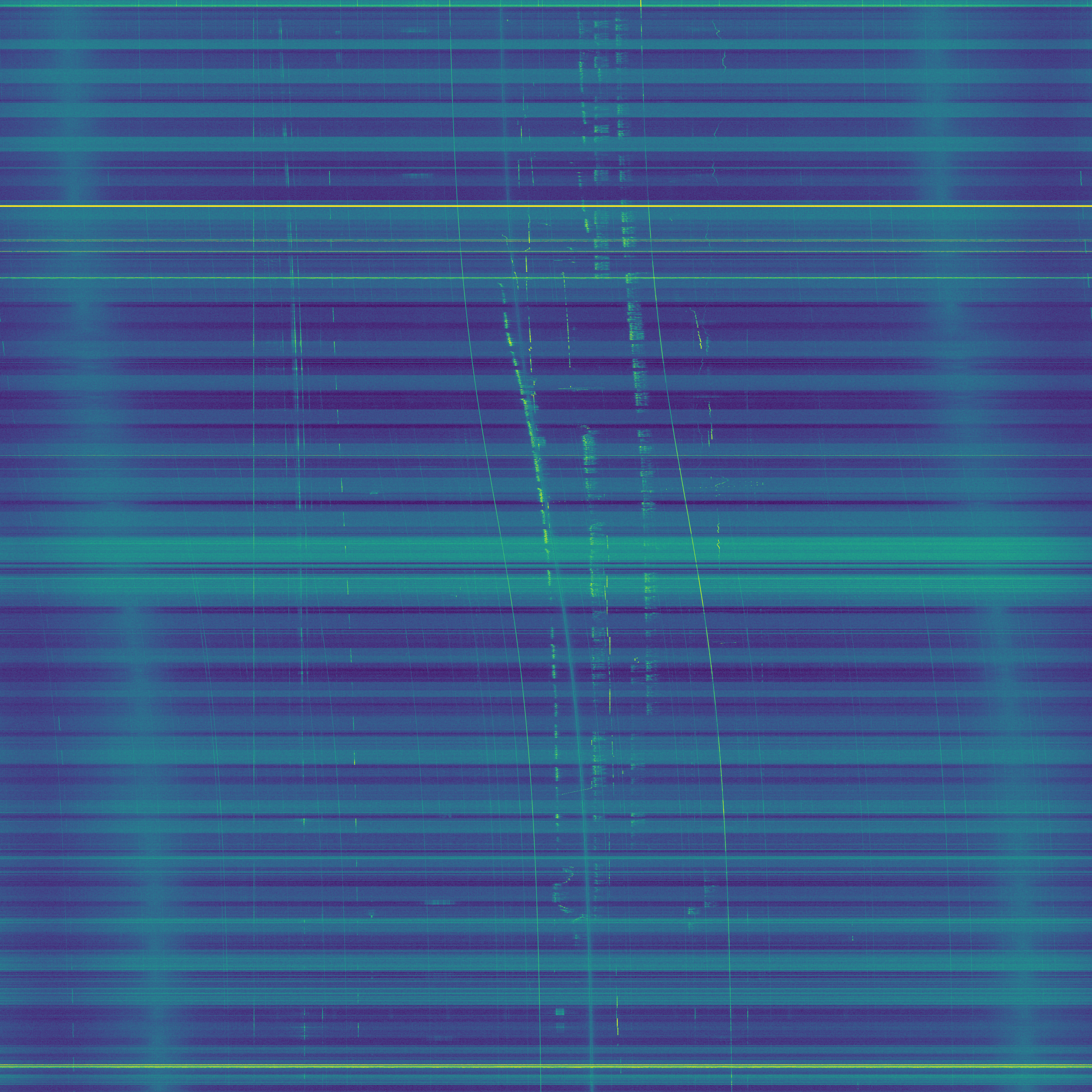
The only transmission that I have managed to decode was made at 18:11 UTC. The two screenshots below show WSJT-X decoding the WAV file extracted from the recording.
WSJT-X decoding the Moonbounce signal
Note the direct signal with a lowest tone at 1800Hz. The reflected signal is very faint, with a lowest tone at 700Hz. The Doppler spread of the reflected signal is large, approximately 200Hz, although it is difficult to judge from the spectrum.
When the WAV file is created, I also compensate for a linear frequency drift of 25Hz per minute due to Doppler, but this is not essential to obtain a valid decode.
WSJT-X decoding the Moonbounce signal
The WAV file that produces a decode can be downloaded here. This file can be opened directly by WSJT-X.
In one of my latest posts I commented on the Moonbounce signal of the Chinese lunar satellite DSLWP-B, as received in Dwingeloo. In the observation made in 2018-10-07 Cees Bassa discovered a signal in the waterfall of the Dwingeloo recordings that seemed to be a reflection off the Moon of DSLWP-B’s 70cm signal. My analysis showed that the Doppler of this signal was compatible with a specular reflection on the lunar surface.
In this post I study the cross-correlation of the Moonbounce signal against the direct signal. This gives some information about how the radio signals behave when reflecting off the Moon. Essentially, we compute the Doppler spread and time delay of the Moonbounce channel.
If you have been following my latest posts, you will know that a series of observations with the DSLWP-B Inory eye camera have been scheduled over the last few days to try to take and download images of the Moon and Earth (see my last post). In a future post I will do a chronicle of these observations.
On October 6 an image of the Moon was taken to calibrate the exposure of the camera. This image was downlinked on the UTC morning of October 7. The download was commanded by Reinhard Kuehn DK5LA and received by the Dwingeloo radiotelescope.
Cees Bassa observed that in the waterfalls of the recordings made in Dwingeloo a weak Doppler-shifted signal of the DSLWP-B GMSK signal could be seen. This signal was a reflection off the Moon.
As far as I know, this is the first reported case of satellite-Moon-Earth (or SME) propagation, at least in Amateur radio. Here I do a Doppler analysis confirming that the signal is indeed reflected on the Moon surface and do some general remarks about the possibility of receiving the SME signal from DSLWP-B. Further analysis will be done in future posts.
In one of my latest posts I analysed the meteor scatter pings from GRAVES on a recording I did on August 11 (see that post for more details about the recording). The recording covered the frequency range from 142.5MHz to 146.5MHz and was 1 hour and 34 minutes long. Here I look at the Amateur stations that can be heard in the recording. Note that Amateur activity in meteor scatter communications increases considerably during large meteor showers, due to the higher probabilities of making contacts.
GRAVES is a French space surveillance radar that transmits with very high power at 143.050MHz. It is easy to receive it from neighbouring countries via meteor scatter. During this year’s Perseids meteor shower I did a recording of GRAVES and the 2m Amateur band for later analysis. The recording was done at 08:56 UTC of Saturday 12th August and it is about 1 hour and 34 minutes long. Here I present an algorithm to detect and extract the meteor scatter pings from GRAVES.
Yesterday I tried to detect DSLWP-B using my 7 element Arrow satellite yagi. The test schedule for DSLWP-B was as follows: active between 21:00 and 23:00 UTC on 2018-06-22. GMSK telemetry transmitted both on 435.4MHz and 436.4MHz. JT4G only on 435.4MHz every 10 minutes starting at 21:10. The idea was to record the tests with my equipment and the run my JT4G detector, which should be able to detect very weak signals. Today I have processed the recorded data and I have obtained a clear detection of one of the JT4G transmissions (albeit with a small SNR margin). This shows that it is possible to detect DSLWP-B with very modest equipment.
In the previous post, I detailed my experiments transmitting FT8 through the FO-29 linear transponder. I recorded a complete pass of the FO-29 satellite while I transmitted an FT8 signal trough the transponder on even periods. As I promised in that post, I have now made a waterfall with the recording to show the activity through the linear transponder, and the strength of my FT8 signal in comparison with the SSB and CW signals of other users.
The watefall can be seen below. You can click on the image to view it in full size. A higher resolution version is available here (24MB). The horizontal axis represents frequency and the vertical axis represents time, with the beginning of the pass at the top of the image. The waterfall has been corrected for the downlink Doppler and the DC spike of the FUNcube Dongle Pro+ has been removed.
From left to right, the following signals can be seen: The CW beacon can be seen as a faint vertical signal. Next, there is some interference coming through the transponder in the form of terrestrial FM signals. Then we can see my FT8 signal, being transmitted only on even periods. Finally, around the centre of the image, we have a few SSB and CW signals through the transponder. Note that most of these signals increase in frequency as the pass progresses. This is because many people keep a fixed uplink and only tune the downlink by hand to correct for Doppler. Unfortunately, full computer Doppler correction is not very popular. I also used a fixed uplink frequency for my FT8 signal, but only to simplify the experiment. The best procedure is to correct for the uplink Doppler to keep a constant frequency at the satellite.
Waterfall of FO-29 downlink (Doppler corrected)
We can see that the SSB and CW signals are much stronger than my FT8 signal. Indeed, some of the CW signals are particularly strong at times, perhaps putting too much pressure on the linear transponder.