vhf & uhf – Page 3 – Daniel Estévez

First FT8 test through FO-29

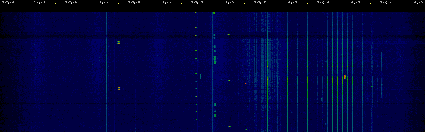
Continuing with my research on using WSJT-X modes through linear transponder satellites in low Earth orbit (see part I and part II), a few days ago I transmitted and recorded an FT8 signal through the V/U linear transponder on FO-29 during a complete pass. The recording started at 2017/10/23 20:26:00 UTC and ended at 20:42:30 UTC. It was made with a FUNcube Dongle Pro+ set to a centre frequency of 435.850MHz and connected to a handheld Arrow satellite yagi through a duplexer. Here the duplexer was used to avoid desense on transmit.

An FT8 signal was transmitted on every even period during the recording, at a fixed frequency of 145.990MHz, using a Yaesu FT-817ND and the Arrow antenna. The signal was transmitted using lower sideband (i.e., inverted in the frequency domain) to get a correct FT8 signal through the inverting transponder. The transmit power was adjusted often to get a reasonable signal through the transponder and avoid using excessive power. There have been reports and complaints of people using too much power with digital modes through linear satellites. In this post, a study of the power is included to show that it is possible to use digital modes effectively without putting any pressure on the satellite’s transponder.

Out of the 33 even periods, a total of 24 can be decoded by WSJT-X using the best TLEs from Space-Track. No measures were taken to correct for the time offset \(\delta\) that has been studied in the previous posts, as the TLEs already provided a good Doppler correction. Regarding the choice of TLEs, there are still some remarks to make. First, the epoch of the TLEs used was 2017/10/23 21:39:16 UTC, so these TLEs were actually taken after the pass. The previous TLEs were taken a few hours before the pass, and it is likely that they also provided a good correction, perhaps by using a time offset \(\delta\) if necessary. However, I do not know if these previous TLEs were also available from CelesTrak before the start of the pass, as it seems that TLEs take a while to propagate from Space-Track to Celestrack. To explain why the TLEs with no time offset correction are enough, it will be interesting to study the rate of change of TLE parameters for FO-29. This will be done in a future post.

The results of this test look very promising. Even though this wasn’t an overhead pass (the maximum elevation was 40º), the maximum rate of change of the Doppler was over 20Hz/s for the self-Doppler seen on the FT8 signal and 35Hz/s for the downlink Doppler seen on the CW beacon. Most of the periods which couldn’t be decoded were near the start or end of the pass. This is the only test that I know of that has decoded FT8 signals in the presence of high rates of change of Doppler. The previous tests by other people were made at low elevations, where the rate of change of Doppler is small. This test has shown that it is possible to get many decodes with high rates of change of Doppler, even using no corrections to the TLEs. Here I continue with a detailed analysis of the recording.

WSJT-X and linear satellites: part II

This is a follow-up to the part I post about using WSJT-X modes through a linear transponder on a LEO satellite. In part I, we considered the tolerance of several WSJT-X modes to the residual Doppler produced by a temporal offset in the Doppler computation used for computer Doppler correction. There, we introduced a parameter \(\delta\) which represents the time shift between the real Doppler curve and the computed Doppler curve. The main idea was that a decoder could try to correct the residual Doppler by trying several values of \(\delta\) until a decode is produced.

Here we examine the effect of TLE age on the accuracy of the Doppler computation. The problem is that, when a satellite pass occurs, TLEs have been calculated at an epoch in the past, so there is an error between the actual Doppler curve and the Doppler curve predicted by the TLEs. We show that the actual Doppler curve is very well approximated by applying a time shift to the Doppler curve predicted by the TLEs, justifying the study in part I.

Acquisition and wipeoff for JT9A

Lately, I have been playing around with the concept of doing acquisition and wipeoff of JT9A signals, using a locally generated replica when the transmitted message is known. These are concepts and terminologies that come from GNSS signal processing, but they can applied to many other cases.

In GNSS, most of the systems transmit a known spreading sequence using BPSK. When the signal arrives to the receiver, the frequency offset (given by Doppler and clock error) and delay are unknown. The receiver runs a search correlating against a locally generated replica signal which uses the same spreading sequence. The correlation will peak for the correct values of frequency offset and delay. The receiver then mixes the incoming signal with the replica to remove the DSSS modulation, so that only the data bits that carry the navigation message remain. This process can be understood as a matched filter that removes a lot of noise bandwidth. The procedure is called code wipeoff.

The same ideas can be applied to almost any kind of signal. A JT9A signal is a 9-FSK signal, so when trying to do an FFT to visually detect the signal in a spectrum display, the energy of the signal spreads over several bins and we lose SNR. We can generate a replica JT9A signal carrying the same message and at the same temporal delay than the signal we want to detect. Then we mix the signal with the complex conjugate of the replica. The result is a CW tone at the difference of frequencies of both signals, which we call wiped signal. This is much easier to detect in an FFT, because all the energy is concentrated in a single bin. Here I look at the procedure in detail and show an application with real world signals. Recordings and a Python script are included.

WSJT-X and linear satellites: part I

Several weeks ago, in an AMSAT EA informal meeting, Eduardo EA3GHS wondered about the possibility of using WSJT-X modes through linear transponder satellites in low Earth orbit. Of course, computer Doppler correction is a must, but even under the best circumstances we cannot assume a perfect Doppler correction. First, there are errors in the Doppler computation because the TLEs used are always measured at an earlier time and do not reflect exactly the current state of the satellite. This was the aspect that Eduardo was studying. Second, there are also errors because the computer clock is not perfect. Even a 10ms error in the computer clock can produce a noticeable error in the Doppler computation. Also, usually there is a delay between the time that the RF signal reaches the antenna and the time that the Doppler correction is computed for and applied to the signal, especially if using SDR hardware, which can have large buffers for the signal. This delay can be measured and compensated in the Doppler calculation, but this is usually not done.

Here we look at errors of the second kind. We denote by \(D(t)\) the function describing the Doppler frequency, where \(t\) is the time when the signal arrives at the antenna. We assume that the correction is not done using \(D(t)\), but rather \(D(t – \delta)\), where \(\delta\) is a small constant. Thus, a residual Doppler \(D(t)-D(t-\delta)\) is still present in the received signal. We will study this residual Doppler and how tolerant to it are several WSJT-X modes, depending on the value of \(\delta\).

The dependence of Doppler on the age of the TLEs will be studied in a later post, but it is worthy to note that the largest error made by using old TLEs is in the along-track position of the satellite, and that this effect is well modelled by offsetting the Doppler curve in time. This justifies the study of the residual Doppler \(D(t)-D(t-\delta)\).

Waterfalls from QB50

In the previous post, I analysed a QB50 recording. Now I have prepared some waterfalls from my recording using the procedure I already described a while ago. The image above is obtained from a 1600×1024 waterfall with a resolution of 2.93kHz or 0.86s per pixel. I have labelled all the satellites and cropped it to a 1600×900 image that now I’m using as my desktop wallpaper.

I have also made a large 14120×16384 image with a resolution of 183.1Hz or 0.1s per pixel. The image can be downloaded here (142MB). I have found the following interesting crops within the large image. Remember that you can click on each image to view it in full size.

The fast fading that I detected in nSIGHT is clearly visible below. Note that the beacon period is almost, but not quite, an integer multiple of the fading period.

In the image below, we can see that SpaceCube is not very stable in frequency. The carrier frequency tends to rise rapidly each time that the transmitter goes on. Also, the overall trend is a frequency increase, counteracting the frequency decreasing effect of Doppler. This excerpt is near the end of SpaceCube’s pass, so the change in Doppler is not so large. The other French satellite, X-CubeSat, also shows a similar behaviour.

SpaceCube frequency instability

AAUSAT-4 usually transmits in 4k8 FSK using CCSDS FEC, but it also transmits a CW beacon sometimes. Both can be seen below.

AAUSAT-4 4k8 FSK and CW

Finally, a couple of CW satellites with interesting behaviour. On the upper part of the image below we can see BeEagleSat with fading. On the lower part, we can see Aalto-2 with its characteristic sidebands.

Fading in BeEagleSat and sidebands in Aalto-2

A tour of QB50

The QB50 project consists in a constellation of cubesats with the goal of studying the thermosphere. The cubesats are built by different universities around the world and each of them carries one of three different scientific instruments. A total of 36 cubesats have been built for the QB50 project. All of them transmit on the 70cm Amateur satellite band. A total of 28 were launched to the ISS on April 18th on the Cygnus CRS-7 resupply ship. Over the last two weeks, they have been released from the ISS. The complete launch schedule and radio information can be found here (note that the launches on May 23rd were delayed due to an unforeseen EVA). Several other non-QB50 cubesats, some of them transmitting in the Amateur bands, have also been released together with the QB50 satellites. This is probably the time that more Amateur satellite have been released at the same time. The satellites have not separated much yet, giving a great opportunity to record a single pass and analyse the telemetry of all the satellites.

A few days after the release of all the 28 QB50 cubesats, on May 29th at 18:25:29 UTC, I made an SDR recording of the complete pass of all the cubesats. The recording spans the 3MHz of the 70cm Amateur satellite band (435-438MHz) and lasts 23 minutes and 08 seconds. It was made from locator IN80do using a 7 element handheld yagi (the Arrow satellite yagi) held in the vertical polarization and a LimeSDR. The gain of the LimeSDR was set to maximum, but no external LNA was used. Here I look at the recording, list the satellites heard, and decode their telemetry.

Testing Opera sensitivity with GNU Radio

Some fellow Spanish Amateur Operators were talking about the use of the Opera mode as a weak signal mode for the VHF and higher bands. I have little experience with this mode, but I asked them what is the advantage of this mode and how it compares in sensitivity with the JT modes available in WSJT-X. I haven’t found many serious tests of what is the sensitivity of Opera over AWGN, so I’ve done some tests using GNU Radio to generate signals with a known SNR. Here I’ll talk about how to use GNU Radio for this purpose and the results I’ve obtained with Opera. Probably the most interesting part of the post is how to use GNU Radio, because it turns out that Opera is much less sensitive than comparable JT modes.

Some measurements of CAS-2T on orbit 25

Last Thursday, a CZ-11 Chinese rocket launched from Jiuquan. Alan Kung BA1DU posted in amsat-bb some minutes after launch saying that this launch contains an Amateur payload: CAS-2T. As it is usual with Chinese Amateur satellites, little information is available publicly and we hadn’t heard about CAS-2T before.

According to BA1DU, CAS-2T is a 2U Cubesat with a CW beacon on 70cm and a V/U FM transponder. The satellite will not separate from the upper stage of the rocket, so it will decay between 10 and 30 days before launch. However, this is not correct. After launch, CAS-2T was identified as object 2016-066E by Mike Rupprecht DK3WN using Doppler measurements. This object is on a 1030km x 500km elliptical orbit, so it will not decay soon. Apparently, due to a problem in the launch, the upper stage of the rocket has being put in this 10 year+ orbit. Indeed, there are radar TLEs for 6 objects from this launch. Four of them are on circular orbits of roughly 500km height, while the other two are on elliptical orbits of 1030km x 500km radius. All of these orbits will last for many years.

Reports of CAS-2T from Amateurs worldwide agree that the CW signal has good strength, but it suffers much fading. Unfortunately, the FM transponder does not function properly. It seems to respond well to an uplink signal, but it doesn’t modulate properly, as if it lacked power or suffered some other problem. On Friday afternoon, I took an SDR recording of the CW and FM signals of CAS-2T during its orbit 25. Here I show some measurements of these signals. The recording was done with a 7 element yagi and a FUNcube Dongle Pro+, and it has been Doppler corrected using the TLE for object 2016-066E, which gives a very good match.

Concurso QSL V-UHF

Today I’ve hiked to Cerro de San Pedro, SOTA summit EA4/MD-020 (1425m), to work in the last national V-UHF contest of the year: concurso QSL. This contest is a bit particular, because it coincides with the IARU-R1 UHF & up contest, so the contacts in the UHF & up bands count for both contests. As always, I’m participating in the 6 hours category with my QRP station: a FT-817ND with 5W and a 3 element yagi on 144MHz and 7 element yagi on 432MHz (the Arrow satellite yagi).

I arrived at the summit at 8:00UTC and worked until the end of the contest, at 14:00UTC, so I could enjoy almost 6 full hours of operation. As expected, after 12:00UTC there where few people left in the contest, as almost everybody had gone for lunch. The map of stations worked is below. Stations in green where worked both on 144MHz and 432, stations in blue where worked only on 144MHz and my operating position is marked in red.

Participation has been perhaps a bit low and propagation was not so good at times, but overall I’m happy with my results, which compare well with other contests this year. I missed some usual stations from the zones EA3 and EA5. I think that propagation to these zones was only open briefly during the contest.

IARU R1 145MHz contest

Today I hiked with all the family to La Najarra, SOTA summit EA4/MD-013 (2122m), to participate in the IARU Region 1 145MHz contest. Unfortunately, for some weird reason very few stations in Spain participate in this contest. My plan was to make a combined contest activity and SOTA activation, making QSOs with whoever was working SSB in the contest, but spending most of the time calling in FM. This gives me the opportunity to contact many more stations, because not many hams have a VHF yagi and SSB radio, but many have a VHF vertical and FM radio. It also gives these local hams the possibility to work a SOTA summit (most SOTA activity is in HF here) and work some DX with a quite basic FM station (100km or more are easy to achieve).

I worked from around 9:30UTC to 11:30UTC. The station was, as usual, an FT-817ND with 5W and an Arrow satellite yagi (3 elements).

I’ve put in the contest log all stations that were able to give me their locator (many hams that work only FM have no clue about what locators are). This is OK with the contest rules. The other stations went only to the SOTA log. Below, you can find the map of contest contacts. I made a total of 17 contacts, but, of course, I can’t put on the map the stations that didn’t know their locator.