On Friday, the Psyche mission launched on a Falcon Heavy from Cape Canaveral. This mission will study the metal-rich asteroid of the same name, 16 Psyche. For more details about this mission you can refer to the talk that Lindy Elkins-Tanton, the mission principal investigator, gave a month ago at GRCon23.
The launch trajectory was such that the spacecraft could be observed from the Allen Telescope Array shortly after launch. The launch was at 14:19 UTC. Spacecraft separation was at 15:21 UTC. The spacecraft then rose above the ATA 16.8 degree elevation mask in the western sky at 15:53 UTC. However, the signal was so strong that it could be received even when the spacecraft was a couple degrees below the elevation mask, so I confirmed the presence of the signal and started recording a couple minutes earlier. At this moment, the spacecraft was at a distance of 18450 km. The spacecraft continued to rise in the sky, achieving a maximum elevation of 32.9 degrees at 16:53 UTC, and setting below the elevation mask on the west at 19:22 UTC. At this moment the spacecraft was 103800 km away. The signal could still be received for a few minutes afterwards, but eventually became very weak and I stopped recording.
Since the recording started only 30 minutes after spacecraft separation, we get to see some of the events that happen very early on in the mission. Most of the observations of deep space launches that I have done with the ATA have started several hours after launch. This Twitter thread by Lindy Elkins-Tanton gives some insight about the first steps following spacecraft separation, and I will be referring to it to explain what we see in the recording.
I intend to publish the recordings in Zenodo as usual, but the platform has been upgraded recently and is showing the following message “Oct 14 12:03 UTC: We are working to resolve issues reported by users.” So far I have been unable to upload large files, but I will keep retrying and update this post when I manage.
Update 2023-10-19: Zenodo have now solved their problems and I have been able to upload the recordings. They are published in the following datasets:
On September 24, the OSIRIX-RExsample return capsule landed in the Utah Test and Training Range at 14:52 UTC. The capsule had been released on a reentry trajectory by the spacecraft a few hours earlier, at 10:42 UTC. The spacecraft then performed an evasion manoeuvre at 11:02 and passed by Earth on a hyperbolic orbit with a perigee altitude of 773 km. The spacecraft has now continued to a second mission to study asteroid Apophis, and has been renamed as OSIRIS-APEX.
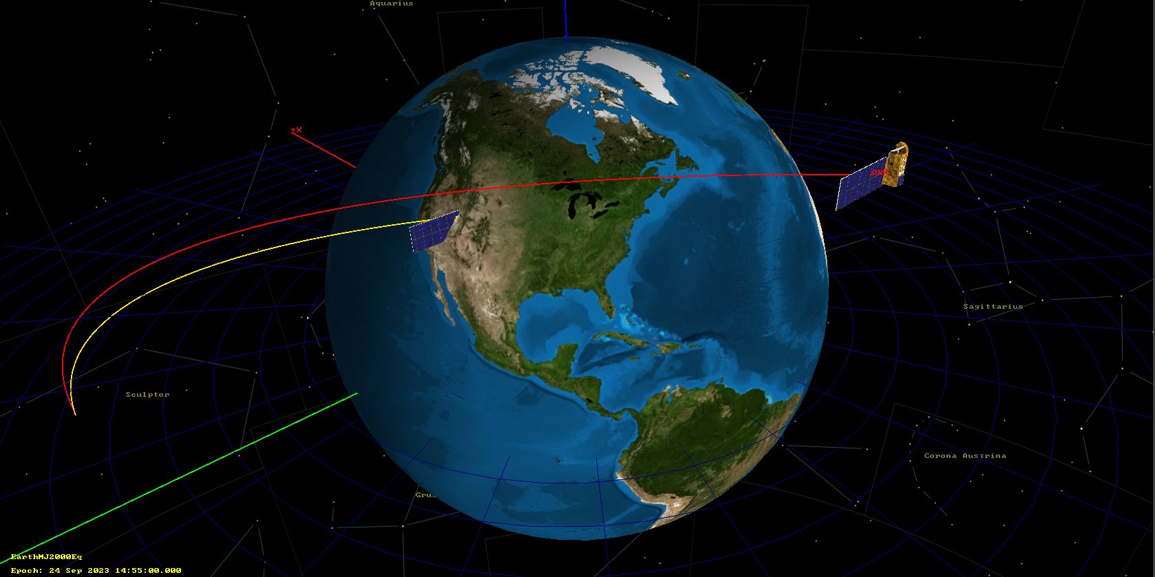
This simulation I did in GMAT shows the trajectories of the spacecraft (red) and sample return capsule (yellow).
Trajectory of OSIRIX-REx and sample return capsule
Since the Allen Telescope Array (ATA) is in northern California, its location provided a great opportunity to observe this event. Looking at the trajectories in NASA HORIZONS, I saw that the sample return capsule would pass south of the ATA. It would be above the horizon between 14:34 and 14:43 UTC, but it would be very low in the sky, only reaching a peak elevation of 17 degrees. Apparently the capsule had some kind of UHF locator beacon, but I had no information of whether this would be on during the descent (during the sample return livestream I then learned that the main method of tracking the capsule descent was optically, from airplanes and helicopters). Furthermore, the ATA antennas can only point as low as 16.8 degrees, so it wasn’t really possible to track the capsule. Therefore, I decided to observe the spacecraft X-band beacon instead. The spacecraft would also pass south of the ATA, but would be much higher in the sky, reaching an elevation above 80 degrees. The closest approach would be only 1000 km, which is pretty close for a deep space satellite flyby.
As I will explain below in more detail, I prepared a custom tracking file for the ATA using the SPICE kernels from NAIF and recorded the full X-band deep space band at 61.44 Msps using two antennas. The signal from OSIRIS-REx was extremely strong, so this recording can serve for detailed modulation analysis. To reduce the file size to something manageable, I have decimated the recording to 2.048 Msps centred around 8445.8 MHz, where the X-band downlink of OSIRIS-REx is located, and published these files in the Zenodo dataset “Recording of OSIRIS-REx with the Allen Telescope Array during SRC reentry“.
In the rest of this post, I describe the observation setup, analyse the recording and spacecraft telemetry, and describe some possible further work.
Aditya-L1 is an Indian solar observer satellite that was launched to the Sun-Earth Lagrange point L1 on September 2. It transmits telemetry in X-band at 8497.475 MHz. This post is going to be just a quick note. Lately I’ve been writing very detailed posts about deep space satellites and I’ve had to skip some missions such as Chandrayaan-3 because of lack of time. There is a very active community of amateur observers doing frequent updates, but the information usually gets scattered in Twitter and elsewhere, and it is hard to find after some months. I think I’m going to start writing shorter posts about some missions to collect the information and be able to find it later.
At the beginning of August I visited the Allen Telescope Array (ATA) for the Breakthrough Listen REU program field trip (I have been collaborating with the REU program for the past few years). One of the things I did during my visit was to use an ADALM Pluto running Maia SDR to do a very quick scan of the radio frequency interference (RFI) on-site. This was not intended as a proper study of any sort (for that we already have the Hat Creek Radio Observatory National Dynamic Radio Zone project), but rather as a spoor-of-the-moment proof of concept.
The idea was to use equipment I had in my backpack (the Pluto, a small antenna, my phone and a USB cable), step just outside the main office, scroll quickly through the spectrum from 70 MHz to 6 GHz, stop when I saw any signals (hopefully not too many, since Hat Creek Radio Observatory is supposed to be a relatively quiet radio location), and make a SigMF recording of each of the signals I found. It took me about 15 minutes to do this, and I made 6 recordings in the process. A considerable amount of time was spent downloading the recordings to my phone, which takes about one minute per recording (since recordings are stored on the Pluto DDR, only one recording can be stored on the Pluto at a time, and it must be downloaded to the phone before making a new recording).
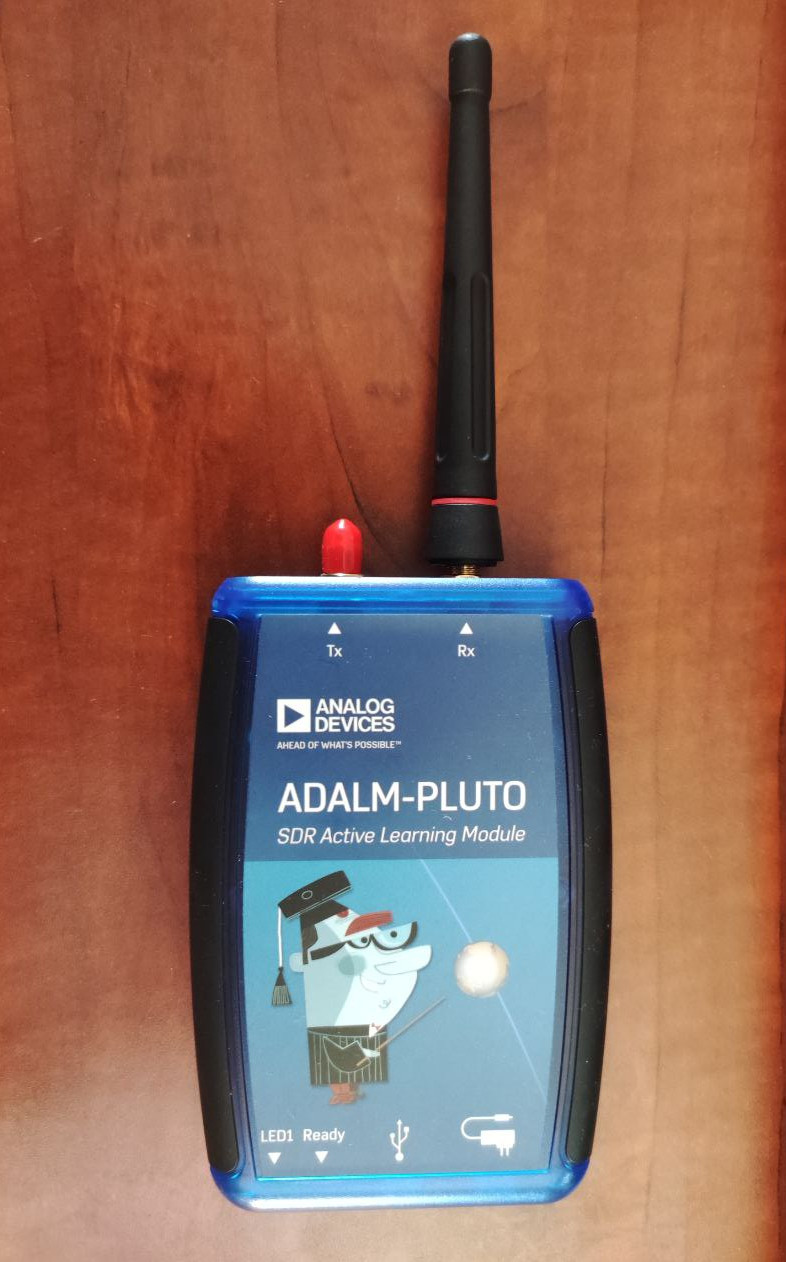
This shows that Maia SDR can be a very effective tool to get a quick idea of how the local RF environment looks like, and also to hunt for local RFI in the field, since it is quite easy to carry around a Pluto and a phone. The antenna I used was far from ideal: a short monopole for ~450 MHz, shown in the picture below. This does a fine job at receiving strong signals regardless of frequency, but its sensitivity is probably very poor outside of its intended frequency range.
ADALM Pluto and 450 MHz antenna
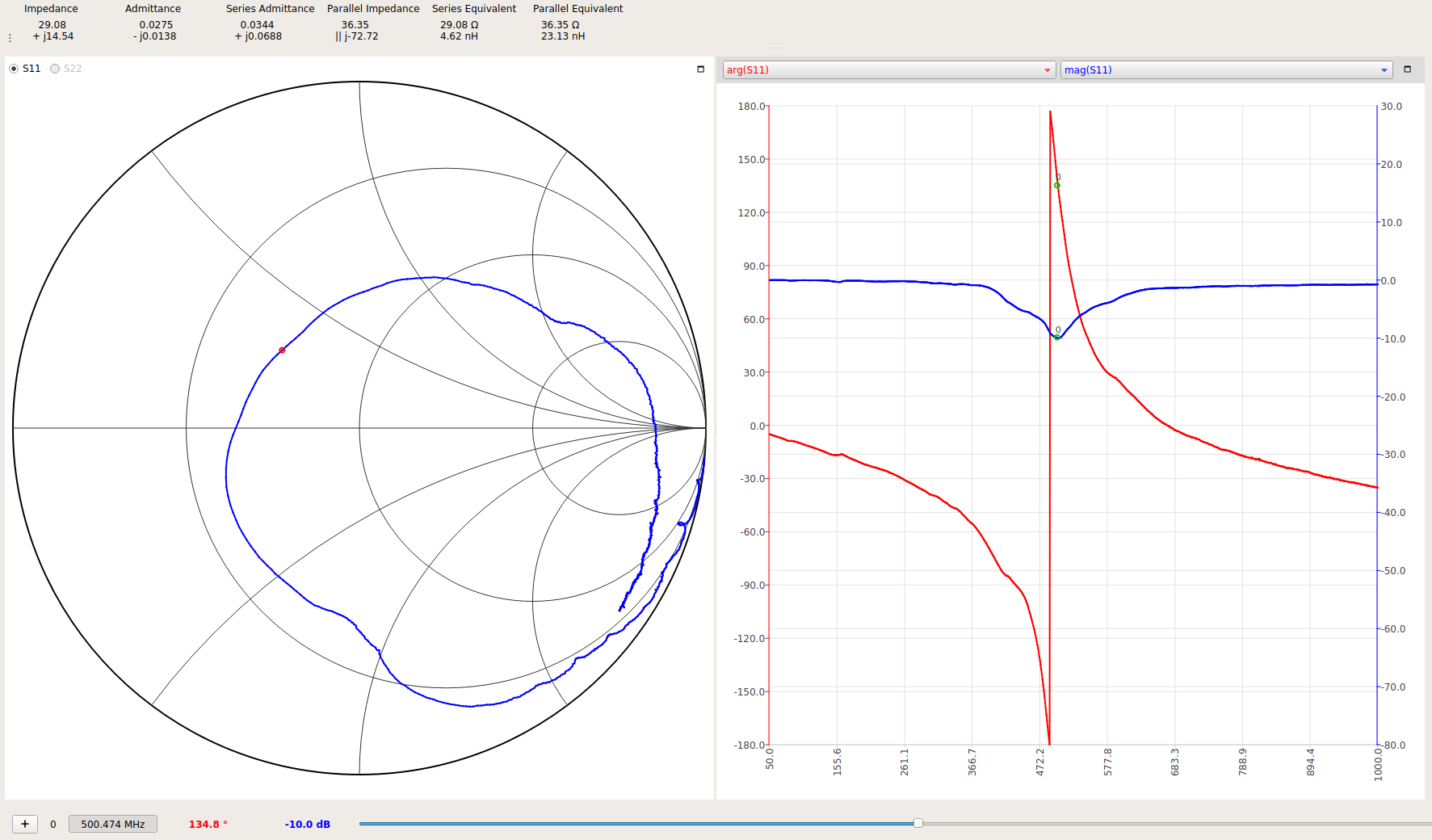
The following plot shows the impedance of the antenna measured with a NanoVNA V2. The impedance changes noticeably if I put my hand on the NanoVNA, with the resonant peak shifting down in frequency by 50 to 100 MHz. Therefore, this measurement should be taken just as a rough ballpark of how the antenna looks like on the Pluto, which I was holding with my hand.
Impedance of the 450 MHz antenna
As the antenna I used for this survey is pretty bad, the scan will only show signals that are actually very strong on the ATA dishes. The log-periodic feeds on the ATA dishes tend to pick up signals that do not bounce off the dish reflectors, and instead arrive to the feed directly from a side. This is different from a waveguide type feed, in which signals need to enter through the waveguide opening. Therefore, besides having the main lobe corresponding to a 6.1 m reflector, the dishes also have relatively strong sidelobes in many directions, with a gain roughly comparable to an omnidirectional antenna. The system noise temperature of the dishes is around 100 to 150 K (including atmospheric noise and spillover), while the noise figure of the Pluto is probably around 5 dB. This all means that the dishes are more sensitive to detect signals from any direction that the set up I was using. In fact, signals from GNSS satellites from all directions can easily be seen with the dishes several dB above the noise floor, but not with this antenna and the Pluto.
Additionally, the scan only shows signals that are present all or most of the time, or that I just happened to come across by chance. This quick survey hasn’t turned up any new RFI signals. All the signals I found are signals we already knew about and have previously encountered with the dishes. Still, it gives a good indication of what are the strongest sources of RFI on-site. Something else to keep in mind is that the frequency range of the Allen Telescope Array is usually taken as 1 – 12 GHz. Although the feeds probably work with some reduced performance somewhat below 1 GHz, observations are done above 1 GHz. Therefore, none of the signals I have detected below 1 GHz are particularly important for the telescope observations, since they are not strong enough to cause out-of-band interference.
I have published the SigMF recordings in the Zenodo dataset Quick RFI Survey at the Allen Telescope Array. All the recordings have a sample rate of 61.44 Msps, since this is what I was using to view the largest possible amount of spectrum at the same time, and a duration of 2.274 seconds, which is what fits in 400 MiB of the Pluto DDR when recording at 61.44 Msps 12 bit IQ (this is the maximum recording size for Maia SDR). The published files are as produced by Maia SDR. At some point it could be interesting to add additional metadata and annotations.
In the following, I do a quick description of each of the 6 recordings I made.
W-Cube is a cubesat project from ESA with the goal of studying propagation in the W-band for satellite communications (71-76 GHz downlink, 81-86 GHz downlink). Current ITU propagation channel models for satellite communications only go as high as 30-40 GHz. W-Cube carries a 75 GHz CW beacon that is being used to make measurements to derive new propagation models. The prime contractor is Joanneum Research, in Graz (Austria). Currently, the 75 GHz beacon is active only when the satellite is above 10 degrees elevation in Graz.
Some months ago, a team from ESA led by Václav Valenta have started to make observations of this 75 GHz beacon using a portable groundstation in ESTEC (Neatherlands). The groundstation design is open source and the ESA team is quite open about this project. I have recently started to collaborate with them regarding opportunities to engage with the amateur radio community in this and future W-band propagation projects (there is an amateur radio 4 mm band, which usually covers from 75.5 to 81.5 GHz, depending on the country). As I write this, some of my friends in the Spain and Portugal microwave group are running tests with their equipment to try to receive the beacon.
On 2023-06-16, the team made an IQ recording of the beacon using their portable groundstation. They have published some plots about this observation. Now they have shared the recording with me so that I can analyse it. One of the things they are interested in is to evaluate the usage of the gr-satellites Doppler correction block to perform real-time Doppler correction with a TLE. So far they are doing Doppler correction in post-processing, but due to the high Doppler drift, it is not easy to see the uncorrected signal in a spectrum plot.
Today is the third anniversary of Tianwen-1, which was launched in 23 July 2020. During the first year of the mission I was tracking it with great detail and writing a lot of posts. A fundamental part of this work was the help of AMSAT-DL. Using its 20 metre antenna in Bochum, they tracked the spacecraft, decoded telemetry and provided live coverage of many of the key mission events in their Youtube livestream. At some point the reception of Tianwen-1’s telemetry at Bochum got completely automated, as we described in a paper in the GNU Radio Conference 2021 proceedings.
To this date, the reception continues in Bochum almost every day, when the dish is not busy with other tasks such as tracking STEREO-A. This means that we get good coverage of the spacecraft orbital data, via the state vectors transmitted in its telemetry.
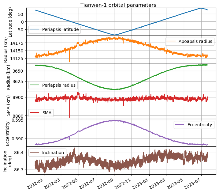
To celebrate the anniversary, I have updated my plot of the orbital parameters, which I made back in March 2022. The plot covers all the remote sensing orbit, from when it started on 8 November 2021, until the present day. To my knowledge, no manoeuvres have happened in this time (perhaps small station-keeping burns would be unnoticed without more careful analysis), so the changes in the orbit are just due to perturbations by forces such as the Sun’s gravity and the oblateness of Mars.
The updated plot can be seen below. We see that the periapsis latitude changes at a steady rate of 0.598 deg/day. The remote sensing orbit was designed so that the periapsis precessed in this way, which allows the spacecraft to cover all the surface of Mars from a low altitude in 301 days. The surface has now been covered twice, since the periapsis has moved from near the north pole to the south pole and back again to the north pole.
There is also an interesting change in eccentricity, which seems to be correlated with the latitude of the periapsis. The eccentricity is largest when the periapsis is over the south pole. In this case, the altitude of the periapsis decreases by 60 km, compared to when the periapsis is over the north pole. The inclination has remained mostly steady, although there seems to be a small perturbation with an amplitude of 0.1 deg.
The updated Jupyter notebook in which this plot was made can be found here.
STEREO-A is a NASA solar observation spacecraft that was launched in 2006 to a heliocentric orbit with a radius of about 1 au. One of the instruments, called SECCHI, takes images of the Sun using different telescopes and coronagraphs to study coronal mass ejections. Near real-time images of this instrument can be seen in this webpage. These images are certainly the most eye-catching data transmitted by STEREO-A in its X-band space weather beacon.
In September 2022, Wei Mingchuan BG2BHC made some recordings of the space weather beacon using a 13 meter antenna in Harbin Institute of Technology. I wrote a blog post showing a GNU Radio decoder and a Jupyter notebook analysing the decoded frames. I managed to figure out that some of the data corresponded to the S/WAVES instrument, which is an electric field sensor with a spectrometer covering 125 kHz to 16 MHz.
During this summer, STEREO-A is very close to Earth for the first time since it was launched. This has enabled amateur observers with small stations to receive and decode the space weather beacon. As part of these activities, Alan Antoine F4LAU and Scott Tilley VE7TIL have figured out how to decode the SECCHI images. Scott has published a summary of this in his blog, and Alan has added a decoding pipeline to SatDump. Using this information, I have now extended my Jupyter notebook to decode the SECCHI images. Eventually I want to turn this into a GNU Radio demo, and the Jupyter notebook serves as reference code.
In a previous post I looked at the modulation and coding of Euclid, the recently launched ESA space telescope. I processed a 4.5 hour recording that I did with two dishes from the Allen Telescope Array. This post is an analysis of the telemetry frames. As we will see, Euclid uses CCSDS TM Space Data Link frames and the PUS protocol version 1. The telemetry structure is quite similar to that of JUICE, which I described in an earlier post. I have re-used most of my analysis code for JUICE. However, it is interesting to look at the few differences between the two spacecraft.
Euclid is an ESA near-infrared space telescope that was launched to the Sun-Earth Lagrange L2 point on July 1, using a Falcon 9 from Cape Canaveral. The spacecraft uses K-band to transmit science data, and X-band with a downlink frequency of 8455 MHz for TT&C. On July 2 at 07:00 UTC, 16 hours after launch and with the spacecraft at a distance of 167000 km from Earth, I recorded the X-band telemetry signal using antennas 1a and 1f from the Allen Telescope Array. The recording lasted approximately 4 hours and 30 minutes, until the spacecraft set.
Even though the telemetry signal fits in about 300 kHz, I recorded at 4.096 Msps, since I wanted to see if there were ranging signals at some point. Since the IQ recordings for two antennas at 4.096 Msps 16-bit are quite large, I have done some data reduction before publishing to Zenodo. I have decided to publish only the data for antenna 1a, since the SNR in a single antenna is already very good, so there is no point in using the data for the second antenna unless someone wants to do interferometry. Since looking in the waterfall I saw no signals outside of the central 2 MHz, I decimated to 2.048 Msps 8-bit. Also, I synthesized the signal polarization from the two linear polarizations. To fit within Zenodo’s constraints for a 50 GB dataset, I split the recording in two parts of 32 GiB each.
In this post I will look at the signal modulation and coding and present GNU Radio decoders. I will look at the contents of the telemetry frames in a future post.
On June 2, ESA celebrated the 20th anniversary of the launch of Mars Express (MEX) by livestreaming images of Mars from the VMC camera in a Youtube livestream. They set things up so that an image was taken by the camera approximately every 50 seconds, downlinked in the X-band telemetry to the Cebreros groundstation, which was tracking the spacecraft, and then sent to the Youtube. The total latency, according to the image timestamps that were shown in Youtube was around 17 minutes, which is quite good, since most of that latency was the 16 minutes and 45 seconds of one-way light time from Mars to Earth.
The livestream was accompanied by commentary from Simon Wood and Jorge Hernández Bernal. One of the things that got my attention during the livestream was the mention that to make the livestream work, the VMC camera should be pointing to Mars and the high-gain antenna should be pointing to Earth. This could only be done during part of Mars Express orbit, and in fact reduced the amount of sunlight hitting the solar panels, so it could not be done for too long.
This gave me the idea to use the Mars Express SPICE kernels to understand better how the geometry looked like. This is also a good excuse to show how to use SPICE.