Since watching Matt Venn‘s video about flip-flop timing, I have had at the back of my mind the idea of designing my own ASIC flip-flop and doing some simulations to measure its timing parameters. This is partly an excuse to learn how to use Magic and other VLSI design tools, and partly a good way to understand better how the numbers that appear on a flip-flop datasheet relate to what physically happens in the flip-flop.
I have now designed a flip-flop in Magic and done ngspice simulations to measure its setup, hold and output delay times. This work can be found in a flip-flop-timing repository in Github. In this post I explain how the flip-flop is designed and how the timing analysis is done.
In February this year I was in the Spanish amateur microwave radio conference Micromeet 2025. In this conference, Luis Cupido CT1DMK presented a simple and inexpensive 10 GHz transverter that he called Nes-Transverter, with the motto “Instant microwaves. Just add solder”. The main idea of this design is that it is very simple and can be built by anyone with just a handful of inexpensive components. Luis was hoping that this project would help more people get on the 10 GHz band in a hands-on way, and he also wanted to demystify some ideas such as amateur microwave radio being difficult or expensive.
The schematic for this design is available here. It uses a 144 MHz IF, allowing it to be connected to a VHF amateur radio. An ADF4351 synthesizer, to be sourced from an inexpensive AliExpress dev board, generates a 2.556 GHz LO with complementary outputs. These two outputs are used in a frequency doubler built with two BAT15 diodes to produce a 5.112 GHz LO, which is filtered with a transmission line stub and amplified with an MMIC such as the ERA 3+. A harmonic x2 mixer built with two BAT15 diodes directly connected to the waveguide probe uses the 5.112 GHZ LO and the 144 MHz IF to produce 10.368 GHz, which is the usual frequency for terrestrial narrowband communications in the 10 GHz amateur band.
I was very interested by this talk, and thought that it would be fun to play with this project, since I haven’t done any hands-on electronics projects in quite a while. However, rather that building a transverter for narrowband communications, I decided to adapt the ideas to build a 10 GHz FMCW radar. I wanted to build a cheaper version of the ADALM-PHASER, minus the phased array part. The Phaser is an educational development kit from ADI that demonstrates concepts in phased array beamforming and FMCW radar. It uses an ADF4159 waveform generator synthesizer and a HMC735 VCO as a 12.2-12.7 GHz LO source that can be programmed to generate FMCW waveforms such as a linear sawtooth and triangle chirps. An ADALM-PLUTO or another SDR is used as a 2.2 GHz IF to obtain 10-10.5 GHz via high-side LO injection. On the transmit section, the 10-10.5 GHz signal is sent to an SMA connector to drive an external antenna. On the receive section, a 4×8 phased array of patches is included in the PCB. Each column of 4 patches is phased as a single element by connecting them together on the PCB. The 8 columns are beamformed in groups of 4 with two ADAR1000, which allows choosing independent complex coefficients for each column. Each of the 4-column beamformer outputs is connected to an RX channel of a 2-channel SDR, so that the final beamforming step can happen in software (see here for a block diagram of the Phaser).
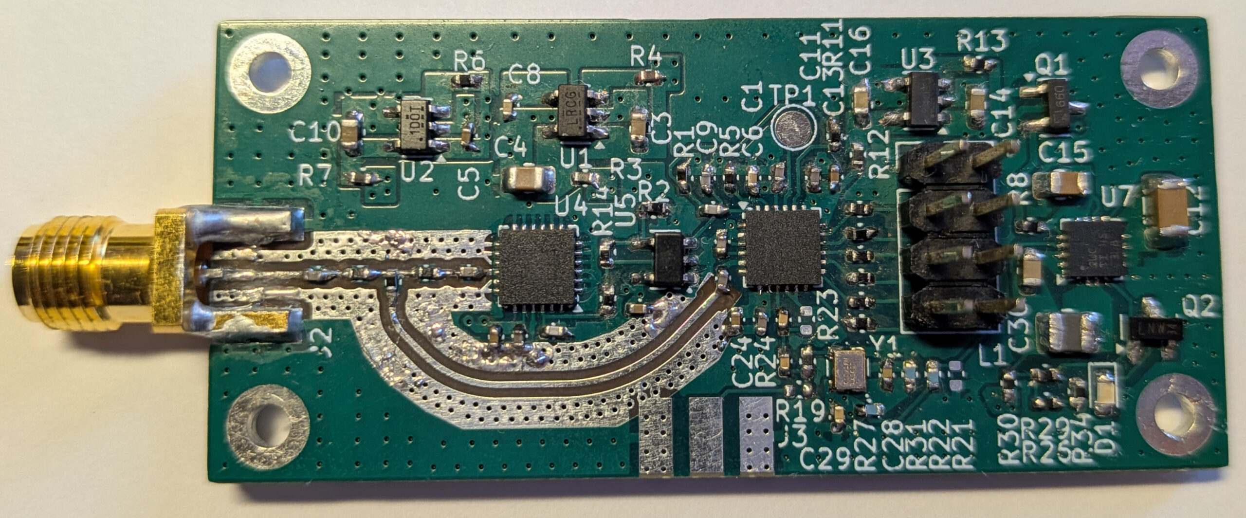
The first thing I needed to replace in Luis design to convert it to an FMCW radar was the LO source. Since I will be using an SDR rather than a VHF radio as the IF, I could use an LO of around 4-4.5 GHz, which would give me around 10-10.5 GHz with an IF around 1-2 GHz. This meant that I could use the ADF4158 synthesizer as the LO source. This is the cheaper variant of the ADF4159, and it only goes up to 6.1 GHz instead of 13 GHz, which is fine for my use case. I needed a VCO to go together with the synthesizer, and after some looking around I decided to use another ADI part, the HMC319, which is a 3.9-4.45 GHz VCO. An IF of 1.6 GHz covers 10-10.5 GHz with an LO of 4.2-4.45 GHz, which is quite appropriate for this VCO choice.
I designed a small PCB with an ADF4158 and HMC391, which I now have built and tested. In this post I explain some of the aspects of the board design and the results of the initial tests.
A few days ago, I posted about a recent wildfire in Tres Cantos, Madrid, Spain, sharing images of Pléiades Neo and Sentinel-2 that showed the extent of the fire. Since the Sentinel-2 data products can be downloaded for free and they include multispectral data covering 13 bands including visible, near infrared and short wave infrared spectrum, I have decided to do an analysis of this data. There are two main goals to this. The first is to learn. I have never done this before. It is an interesting topic, and I mostly learn by doing. So bare with me that although all my results seem to make sense, I could have made some mistakes or done something in a suboptimal way.
The second is to understand how badly the holm oak woodland in “Monte de Viñuelas” has been burnt. In the previous post I explained that this is a 30 km² estate and that a large part of it has been hit by the fire. From the wall that borders the estate I can see that the oaks that are near the wall have not burnt, but the grass in the ground has burnt completely. The leaves on these oaks are mostly fine. Some of them might wither with time if the fire has killed the tree (in some previous smaller fires I have seen that if the fire has killed only part of the tree, just that part will wither). Here are some images published by a hunting journal showing how some of these areas look like a few days after the fire.
However, deeper into the woodlands there seems to be more damage and trees burnt completely. This is not so easy to see from the wall, and I cannot just walk in, as it is private land. Aerial photography would be best, but without it, satellite imagery is the next best thing. It is hard to tell how large the damage is from the visible spectrum imagery, but as we will see in this post, the infrared bands have much more information.
This post is going to be slightly unusual for the topics of this blog, because there is no RF, but nevertheless there is space-based remote sensing, which fits somewhat well with the things I usually write about. I wanted to write down this information somewhere, and it was too long for a series of tweets.
As some of you might have heard in the news, there has been a large wildfire in Tres Cantos, Madrid, Spain, which is the city where I live. This has even been featured in international news. First of all, I am okay, as are all the family and friends I have in the city. The fire broke out on 2025-08-11 17:45 UTC (19:45 local time) and by the next morning its perimeter was already contained. As of writing this post on the morning of 2025-08-13, the fire is almost put out and is considered to be controlled. We have been lucky that a fire so close to the city has caused relatively low damage. I am not keeping a tally, but what I heard is: one person’s life, a few houses in the borders of the city, as well as a few countryside houses and sheds, the King’s College British school, and the 17th century Viñuelas castle, as well as part of the castle grounds, which consist of 3000 hectares of holm oak woodland, commonly known as “Monte de Viñuelas”.
Since I woke up on the morning of 2025-08-12, I have been very interested in understanding which area has been affected by the fire. The information I could see in Google maps, and even in some news articles (which could have been based off Google maps) didn’t quite match what I had seen in pictures and videos shared in social media, as well as what I saw by driving on the streets bordering the town. An official map has not been published, as far as I know. So I have been keeping an eye on space-based imagery platforms to see when the first images taken on 2025-08-12 would pop up. I don’t use these services frequently, so this has also helped me get up to speed on the current constellations, platforms and services. This is the topic of this post.
In my last post about 5G NR, which was part of a series in which I analyzed the signals in a short recording of an idle srsRAN gNB, I mentioned that I had already decoded all the signals that appear in the recording, and that to move on with my 5G series I would need to make and use some more complex real world recordings next.
A 5G band I’m particularly interested in is n78 (3.3 – 3.8 GHz TDD). This is being used to deploy 5G in many European countries, including Spain, as showed by this list in Wikipedia. Due to the large bandwidth available, it is common to see cells with 100 MHz bandwidth in this band.
On July 4, an OSNMA live test notification went out with the following message:
EVENT DESCRIPTION: USERS ARE ADVISED THAT, AS PART OF THE PUBLIC OBSERVATION TEST PHASE ACTIVITIES, A TESLA CHAIN RENEWAL IS PLANNED ON 2025-07-07 10:00 UTC AND THE TRANSITION WILL OCCUR ON 2025-07-08 10:00 UTC. THE TESLA CHAIN RENEWAL PROCESS IS DESCRIBED IN THE OSNMA SIS ICD (LINK).
NOTE THAT USER RECEIVERS SHALL PREVENT THE USE OF ANY CHAIN THAT HAS BEEN SUBJECT TO A RENEWAL PROCESS.
Using band-edge filters for carrier frequency recovery with an FLL is an interesting technique that has been studied by fred harris and others. Usually this technique is presented for root-raised cosine waveforms, and in this post I will limit myself to this case. The intuitive idea of a band-edge FLL is to use two filters to measure the power in the band edges of the signal (the portion of the spectrum where the RRC frequency response rolls off). If there is zero frequency error, the powers will be equal. If there is some frequency error, the signal will have more “mass” in one of the two filters, so the power difference can be used as an error discriminant to drive an FLL.
Recently I was looking into band-edge FLLs and noticed some problems with the implementation of the FLL Band-Edge block in GNU Radio. In this post I go through a self-contained analysis of some of the relevant math. The post is in part intended as background information for a pull request to get these problems fixed, but it can also be useful as a guideline for implementing a band-edge FLL outside of GNU Radio.
Z-Sat is a microsatellite by Mitsubishi Heavy Industries that was launched in 2021. It is a demonstrator for multi-wavelength infrared Earth observation technologies. It carries an amateur radio payload that was coordinated by IARU and which consists of a BBS (bulletin board system) with a 145.875 MHz downlink and 435.480 MHz uplink. I have not been able to find more information about the amateur radio payload on this satellite.
Recently, Daniel Ekman SA2KNG asked me to analyze some transmissions by this satellite. Apparently it has recently begun to transmit a digital modulation, as shown in this SatNOGS observation, while it typically had transmitted CW telemetry in the past. The point where this started appears to be on 2025-06-20, as there is a SatNOGS observation of CW telemetry on that day followed by an observation of the digital modulation. In this post I analyze this digital modulation and explain what it is.
In my previous post in the 5G NR RAN series, I showed how to decode the PDCCH (physical downlink control channel), which is used to send control information from the gNB (base station) to the UEs (cellphones). In this series I am using as an example a short recording of the downlink of an srsRAN gNB. The PDCCH transmission that I decoded in the previous post was a DCI (downlink control information) containing the scheduling of the SIB1 PDSCH transmission. The PDSCH is the physical downlink shared channel, which is the channel where the gNB transmits data. The SIB1 is the system information block 1. It contains basic information about the cell, and it is decoded by the UE after decoding the MIB in the PBCH, as part of the cell attach procedure. In this post I will show how to decode this PDSCH SIB1 transmission.
This is a new post in my series about the 5G NR RAN. As in previous posts, I am analyzing a short recording of the downlink of an srsRAN gNB. There are no UEs connected to the cell during this recording, so there isn’t much interesting traffic, but the recording contains all the essential 5G signalling. In particular, there is a SIB1 transmission in the PDSCH, with its corresponding transmission in the PDCCH.
The PDCCH (physical downlink control channel) is used to transmit control information to the UEs in the form of DCI messages (downlink control information). The most common types of DCIs are those that specify the scheduling parameters of transmissions in the PDSCH (physical downlink shared channel), and the uplink grants for UEs in the PUSCH (physical uplink shared channel). The role that the 5G PDCCH plays is very similar to the role that it plays in LTE, so my post about the LTE PDCCH can be good for more context. However, in 5G the channel coding and physical layer of the PDCCH is substantially different from LTE.