Each GNSS system uses their own timescale for all the calculations. What this means is slightly difficult to explain, since anything involving “paper clocks” is conceptually tricky. In essence, the system, as part of the orbit and clock determination, maintains a timescale (paper clock) to which the ephemeris are referenced. This timescale is usually related to some atomic clocks in the countries that manage the GNSS system, and these clocks often participate in the realization of UTC, so that in the end this GNSS timescale is traceable to UTC. For instance, GPS time is related to UTC(USNO), and GST, the Galileo system time, is related to a few atomic clocks in Europe that are realizations of UTC.
Since all the information for a single GNSS system is self-consistent with respect to the timescale it uses, a receiver using a single system to compute position and velocity does not really care about the GNSS timescale. Everything will just work. However, when the receiver needs to compute UTC time accurately (for instance to produce a 1PPS output that is aligned to UTC) or to mix measurements from several GNSS systems, then it needs to handle the different GNSS timescales involved, and transfer all the measurements to a common timescale (and in the case of measuring UTC time or producing a 1PPS output, relating this timescale to UTC).
As part of their broadcast ephemeris, GNSS systems broadcast an estimate of the offset between the system timescale and UTC (this estimate is just a forecast; the true value of UTC is only known a posteriori, when the BIPM publishes its monthly Circular T). Additionally, some systems also broadcast the offset between their timescale and the timescale of another system. For example, Galileo broadcasts the offset GST-GPST, the difference between Galileo system time and GPS time. This is intended as a help to receivers that want to combine measurements from both systems. However, these values are somewhat inaccurate, so it is common for receivers to ignore them, and determine the offsets on their own (this is done by adding extra variables called intersystem biases to the system of equations solved to obtain the navigation solution). This trick only works for combining measurements of different systems. In the case of UTC, receivers do not have any way of directly measuring UTC, so they must trust the broadcast message. Alternatively, some receivers offer an option to align their 1PPS output to a GNSS timescale such as GPST.
These days, most GNSS systems, including GPS and Galileo usually keep their timescales within a few nanoseconds of UTC. According to the specifications of each system, the relation to UTC is much loose. GPS time promises to be synchronized to UTC(USNO) with a maximum error of 1 microsecond. GLONASS time only promises 1 millisecond synchronization to UTC. GST is supposed to be within 50 ns of UTC, and Beidou time within 100 ns. However, if timekeeping is done correctly, there is no reason why the GNSS timescale should drift from UTC by more than a couple nanoseconds (which is the typical drift of physical realizations of UTC). Receivers should assume that the offsets can be as large as the maximum errors in the specification, but might occasionally freak out if they see an offset which is large, either because of bugs if this case was never tested, as in practice the offsets are typically small, or because it suspects an error in its own measurements.
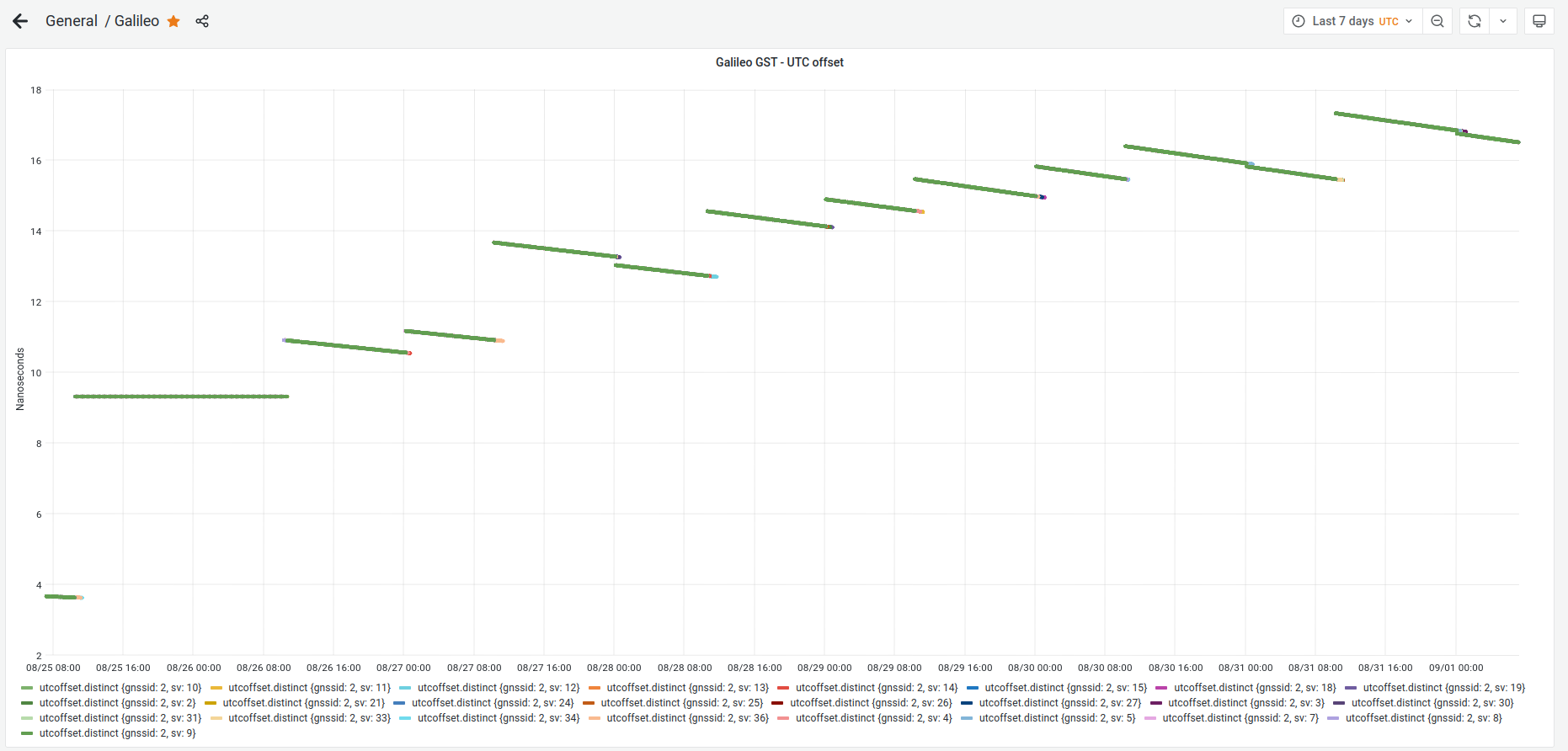
A few days ago, some people in the time-nuts mailing list, and Bert Hubert from galmon.eu noticed that the GST-UTC, the difference between Galileo system time and UTC, had increased to 17 ns and remain around this value during the end of August. This is highly unusual, because GST-UTC is usually smaller than 2 or 3 ns.
galmon.eu provides a public Grafana dashboard where this anomaly can be seen, though the dashboard (or web browser) tends to choke if we request to plot more than one week worth of data.
When hearing about this on Friday, I got interested and commented some ways in which this could be researched further. I also wondered: is the GST-UTC offset actually large, or is it just that the offset estimate in the navigation message is wrong? In this post I explore one of my ideas.
Since here we are setting off to study the GST timescale, which is a paper clock that cannot be measured directly, let me make a conceptual remark first: a GNSS timescale only manifests itself in the broadcast message. Maybe some other GNSS experts will disagree with this claim and say that the timescale is also fundamental in some other processes (I would love to hear these other points of view). What I mean by my comment is that in essence a GNSS system is a bunch of orbiting free-running atomic clocks. We can completely ignore the whole broadcast ephemeris thing and the timescale used by the system and run our own orbit and clock determination referenced to the timescale we like. This is is what the precise orbit and clock products determination does.
In this post I will use the Galileo OS broadcast clock bias as a proxy for the GST timescale. These biases are the offsets between the satellite clocks, which are directly observable physical clocks, and GST, which is a paper clock. I will compare these clock biases with the precise clock products obtained by CODE. These precise clock products use the GPS timescale.
With this comparison, we are actually studying the GST-GPST offset (or the offset between GST and CODE’s idea of GPST). As one can imagine, the GST-GPST offset has also become large, since GPST is still within a couple ns of UTC. Nevertheless, ideally we should make sure of what is the offset between GPST and UTC. The exact value is not known until a month later, as it appears in the BIPM Circular T. For example, in July’s Circular T we can see that the offset between UTC and GPST was beetween -2.2 and 1.8 ns throughout July. Something like this should be expected for August.
The following figure shows the difference between the Galileo OS broadcast clock biases and the CODE precise clock biases. The trace for each satellite is shown in grey, and the average of all these traces is shown in red. We can see that until around 2023-08-20 the offset stays within a couple ns. Then it starts decreasing until reaching around -18 ns. The reason that this plot shows a negative bias is due to how the satellite clock biases are defined. The plot is measuring GPST-GST rather than GST-GPST.
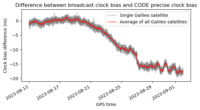
To make this plot I have used the IGS BRDC broadcast ephemeris RINEX files for days 225 (2023-08-13) to 244 (2023-09-01). I’m being careless and not distinguishing between the FNAV and INAV broadcast clocks in the broadcast ephemerides, but this doesn’t seem to matter much, and we would also get into a deep rabbit hole if we consider how this distinction matters for the precise clocks. For the precise clock data I’m using the CODE COD0MGXFIN final solution until day 238 (2023-08-26), and then the COD0OPSRAP rapid solution, since the final solution is not available yet.
We see that this plot indeed confirms that the GST has moved away from UTC by about 18 ns, and is currently staying there.
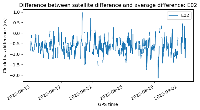
The Jupyter notebook I’m using also contains a plot for each satellite showing the difference between its corresponding grey line and the average (red line). This shows that nothing weird is happening with any of the satellites and also shows the data availability for each satellite (there are some time segments for which there is no data for that particular satellite in the BRDC files). The plots look like this.
The other piece of data we can study is the various GST-UTC, GST-GPST and GPST-UTC offsets that are transmitted in the broadcast messages. RINEX is not a great format to capture this data, because only a single entry of each of these offsets can appear in a daily RINEX file. The rationale for this is that these parameters are updated infrequently (tens of hours) in the navigation message, and that their values change slowly enough that we can use the same entry (taking into account the drift parameter) for all the day. Here this is somewhat limiting, because we would like to do an analysis as fine as possible. Another small inconvenience is that Georinex, which I’m using to parse the RINEX files, doesn’t handle these entries, so I have written my own crude parser.
Using this data I have made the following plot. The red line from the plot above is now plotted in grey, with the opposite sign, for comparison. The offset for each system time difference is shown with a small circle at the corresponding epoch. The drift (which is also included in the navigation message) is shown as the slope of a line with a duration of one day and centred in the circle for the offset. Note that the green lines look very similar to the galmon.eu Grafana data shown at the beginning of the post (I think galmon is doing a very similar thing with the drift).
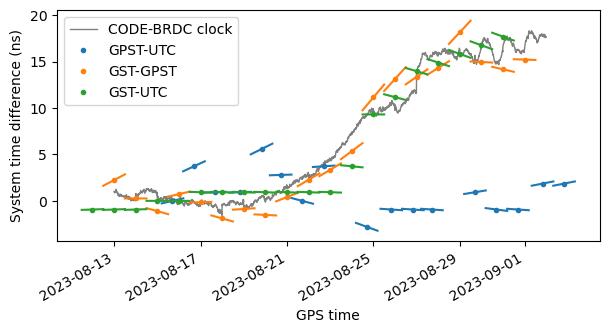
We see that, as expected, the broadcast GPST-UTC difference is small. The GST-GPST and GST-UTC grow following the CODE-BRDC clock measurement, so the offset estimates in the navigation data look correct. However, there is something amiss in the GST-UTC drift data, which Bert Hubert remarked first: the drift of GST-UTC seems to have the opposite sign from what it should. To make this more apparent, I have inverted the sign of the GST-UTC drift and redone the plot. Now the green segments connect together more nicely.
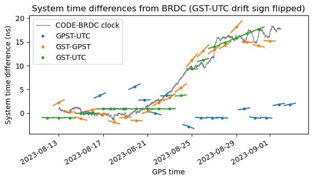
So the GST-UTC drift definitely looks like a bug in the navigation message. This is the kind of bugs that never get tested, because the GST-UTC offset usually never wanders too far away from zero, so the drift is small and almost meaningless.
Besides this bug, the obvious question now is: does any of this matter? As remarked above, GST is only specified to be within 50 ns of UTC, so the current situation is nominal and the receivers should cope with it (but I wouldn’t be surprised if some don’t if the offset keeps growing). On the other hand, this situation is certainly anomalous, and it would be interesting to get more details about how or why it has happened and how does the system plan to recover and steer GST closer to UTC back again.
The Jupyter notebook used in this post can be found here.
2 comments